Part 1: Introduction and Big Ideas: Abstraction and Generalization
Introduction
If you’re a computer science student, you probably had to take an introductory discrete math course at some point. Did you enjoy it? If so, this talk probably isn’t for you, so you can feel free to skip the rest. (Or not – hopefully you feel like you can still learn something from me!)
Jokes aside, it’s actually okay not to enjoy your intro to discrete math course: like, personally, I loved mine, but I also completely hated my discrete probability course and would prefer never to see it again. But I pick on discrete math because I feel like if it’s taught well, it can be a turning point for many people, and it certainly was for me.
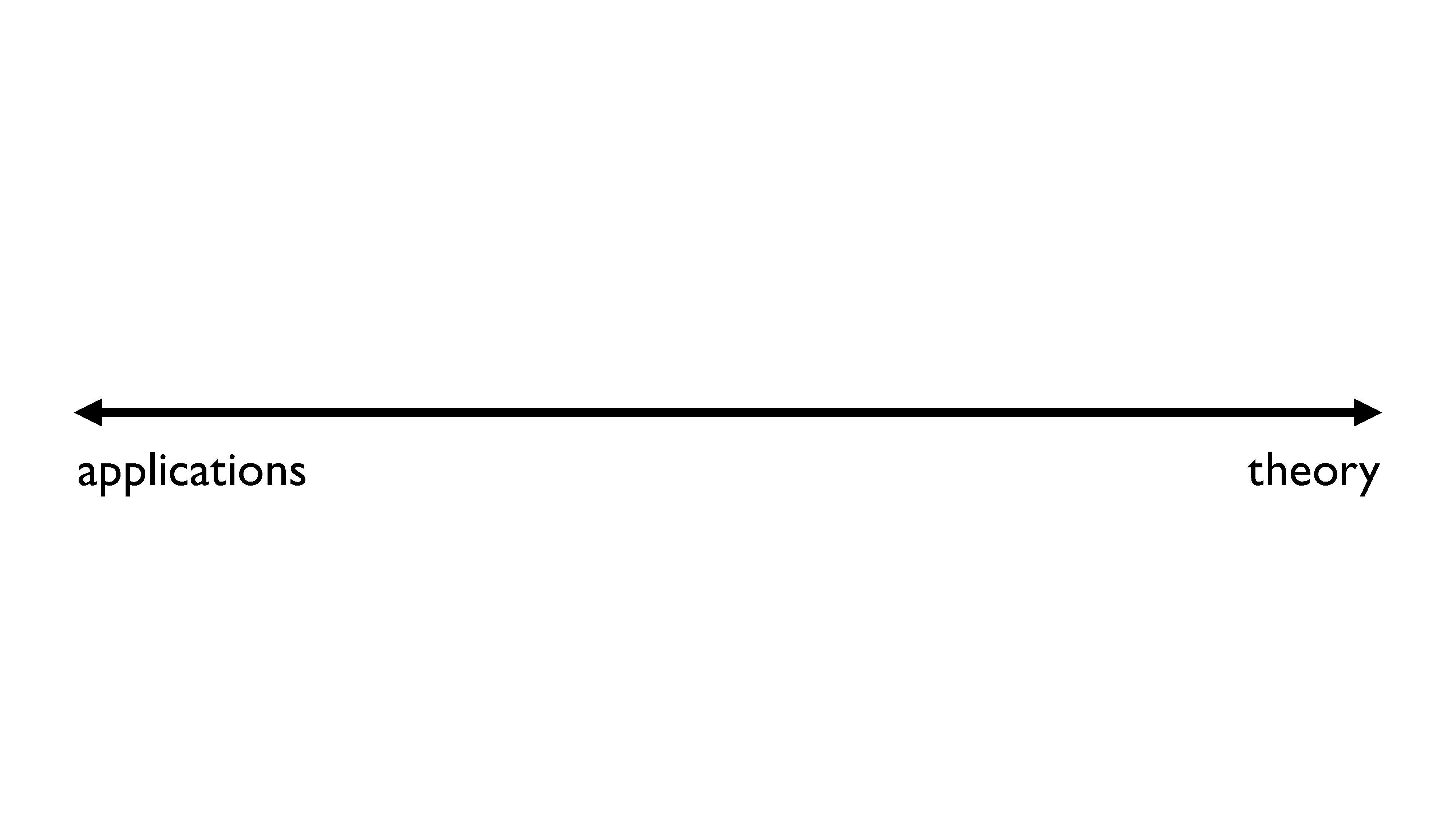
Let’s imagine for a second that everyone falls on this sort of spectrum. On one side, we have people who only care about applications, and on the other side, we have people who only care about theory.
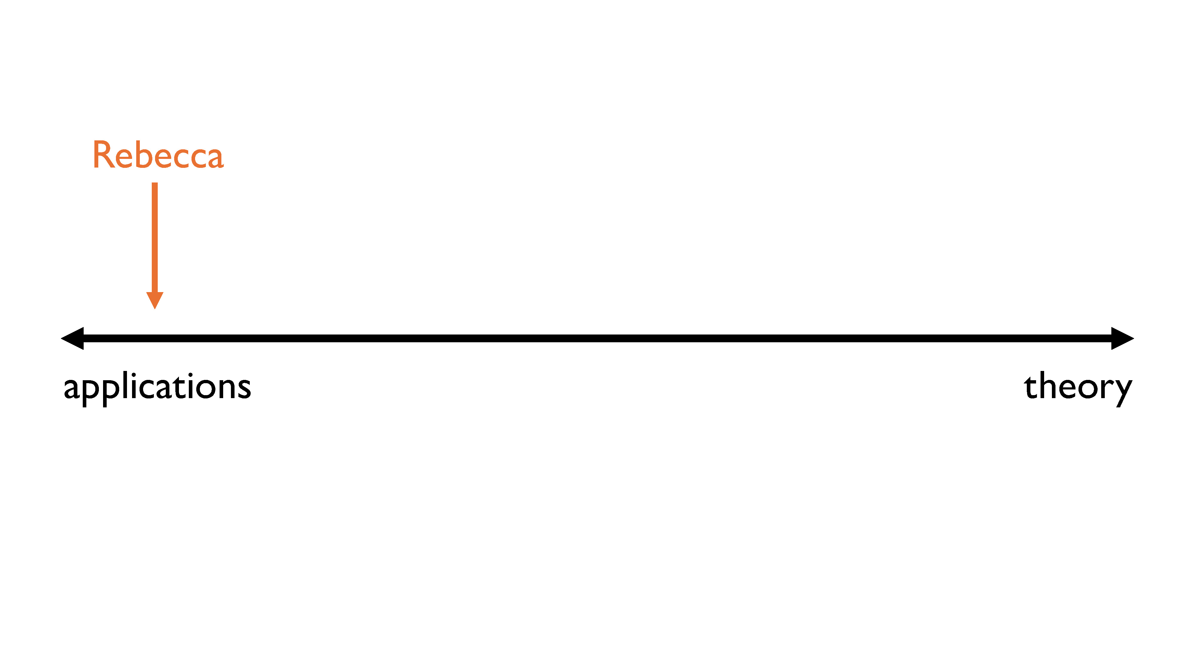
Before I took discrete math, and especially during high school, I fell on the “only cares about applications” side of the spectrum. I knew math was useful, but I didn’t care about it. Actually, I hated it and viewed it as necessary suffering. I went into an engineering program straight after high school, and engineering degrees are all about applications. I only wanted to learn math that I could see a concrete use for, and I was fully planning on never taking a math course again after fulfilling my requirements.
I ended up switching to a computer science degree almost by accident (it’s a long story), and discrete math was certainly the course that opened my eyes to what math really is, why we care about it, and how we can use it to solve problems. After finishing the course, I felt as though the entire field of math had been completely misrepresented to me, and I had a much better understanding of why people study math and how it can be useful in and of itself.
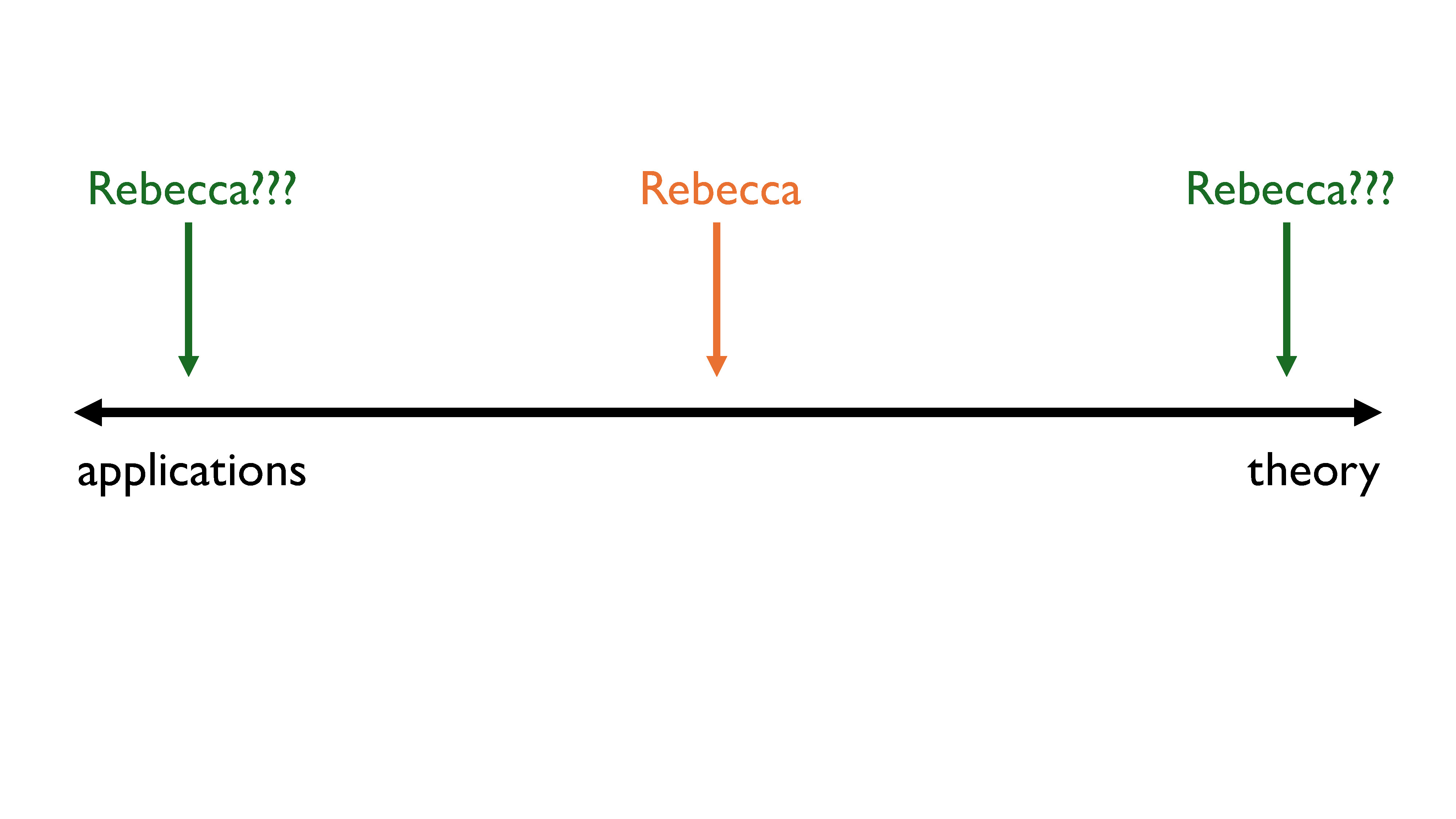
And now I keep taking all these math courses, people keep thinking I’m a math student (which is kind of insane – have you ever met real math students??) and I have a much greater appreciation for theoretical approaches than I used to. Nowadays, I fall more in the middle of this chart, and I think I’ve mostly settled there… with a few wild pendulum swings back and forth.
But that chart is actually a lie.
Theory vs. Applications
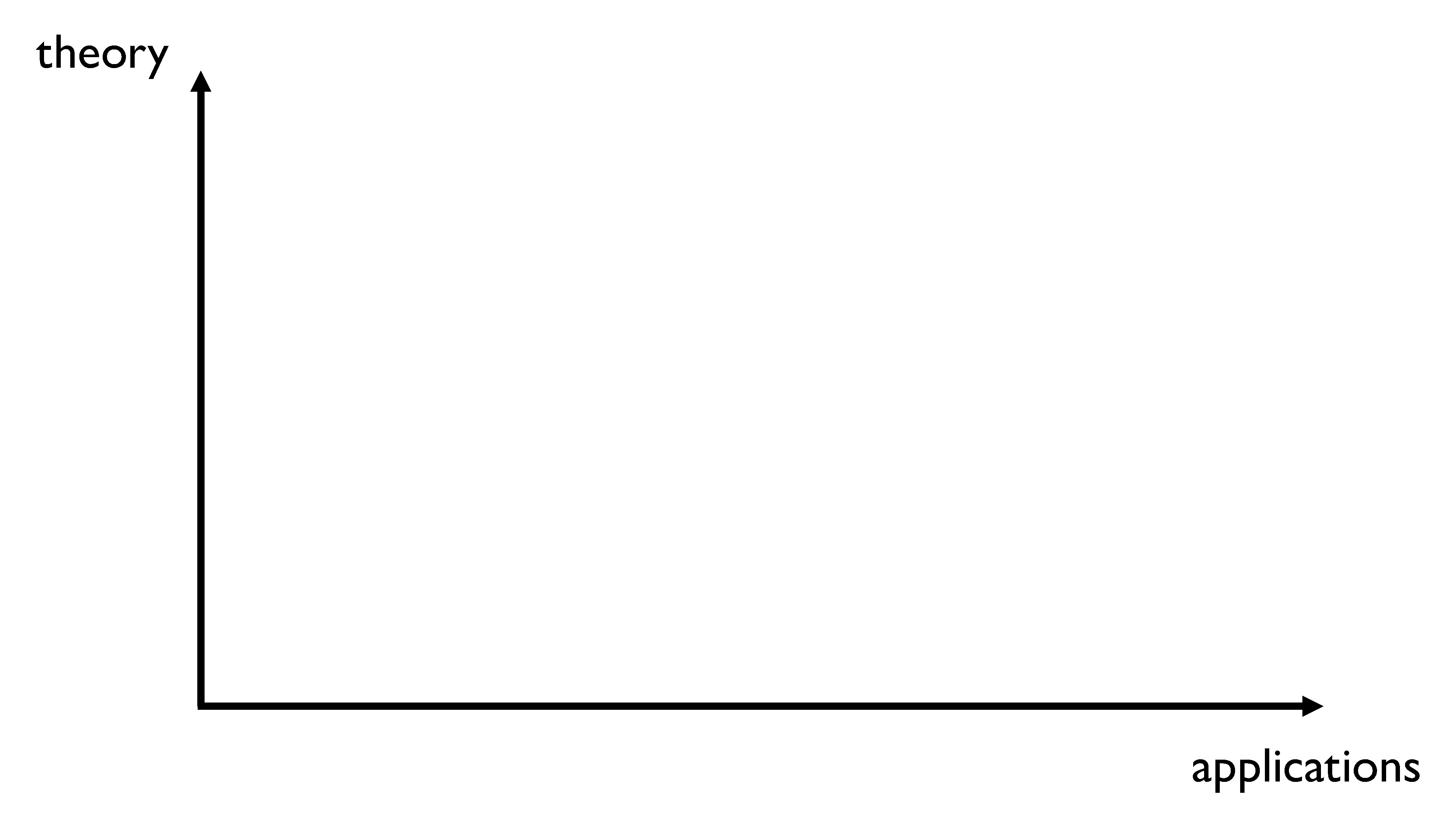
Theory and applications are not separate from each other, so we can start to place courses, professions, and different people’s interests on a two axis chart that looks a lot more like this.
In the bottom left corner, we have things that have no practical or theoretical value. If you’re doing one of those things in a professional or academic context, you should just stop, because it’s stupid and useless and no one is going to care about it. In the top right corner, we have things that have both high theoretical value and high practical value. And again, there are probably very few people who are doing things like that, because most people have more of an inclination towards one of theory or application, both in terms of ability and in terms of interest.
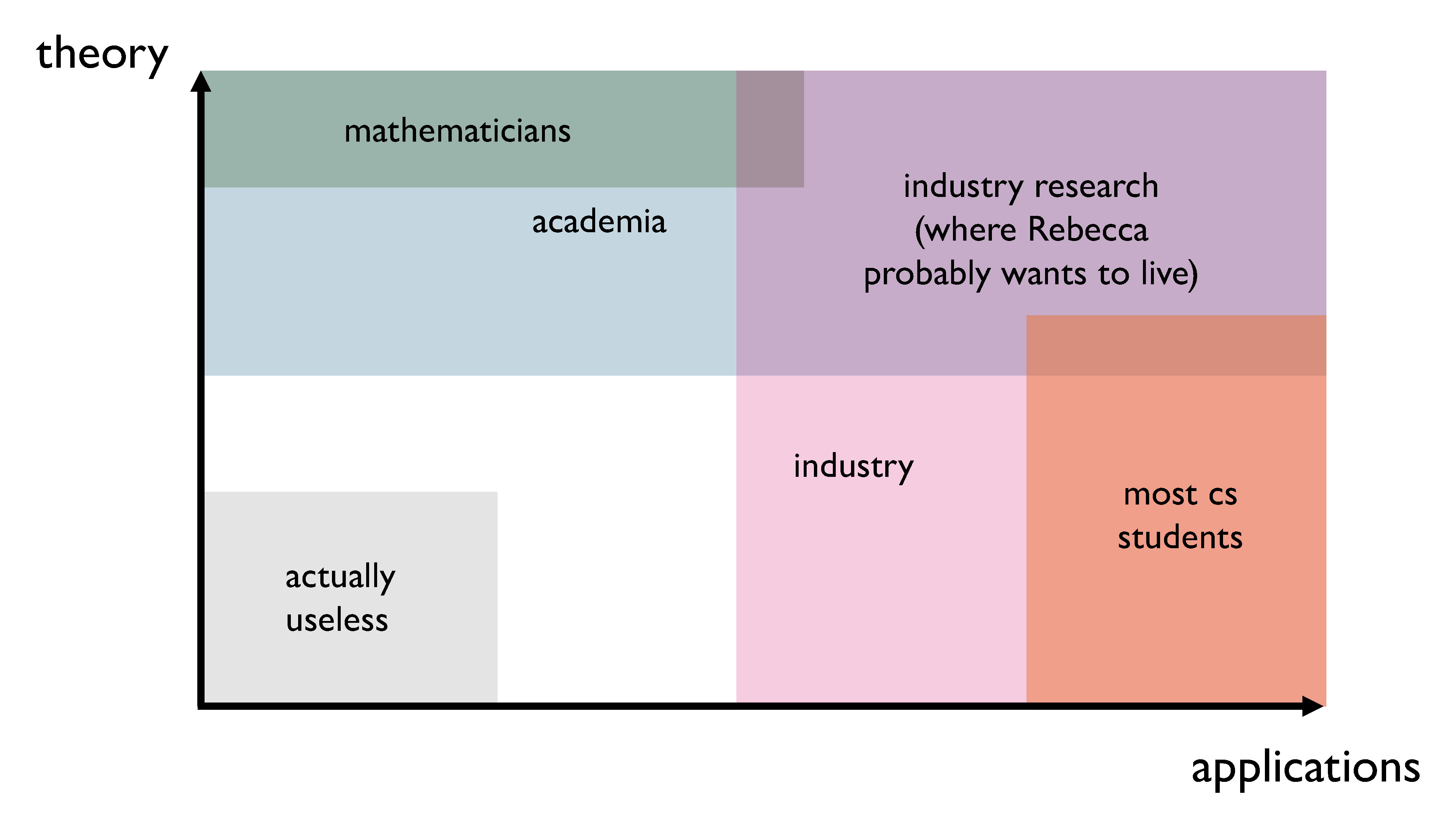
In academia, most people fall into the top half of the chart, because all research involves a theoretical framework and approach. Some of the research may have practical applications, sure, but what academia really values is trying to further knowledge in some way, which usually involves having a firm grounding in theory, or even proposing new ideas and methods. (You’ll notice that pure mathematicians are like, way over in the top left). In industry, most people fall into the right half of the chart, because getting concrete results that are actually useful to the business is of utmost importance. In the intersection of the two areas is where you find industry research, which is where I think I might want to live.
I think most students in computer science programs fall somewhere in the bottom right corner of the chart. We can start to place some different CS courses on this chart, and get a better sense of what the theory/applications split actually looks like in a CS degree. I’ve put a few of the courses I’ve taken on the slide that follows, in the places where I think they actually belong.
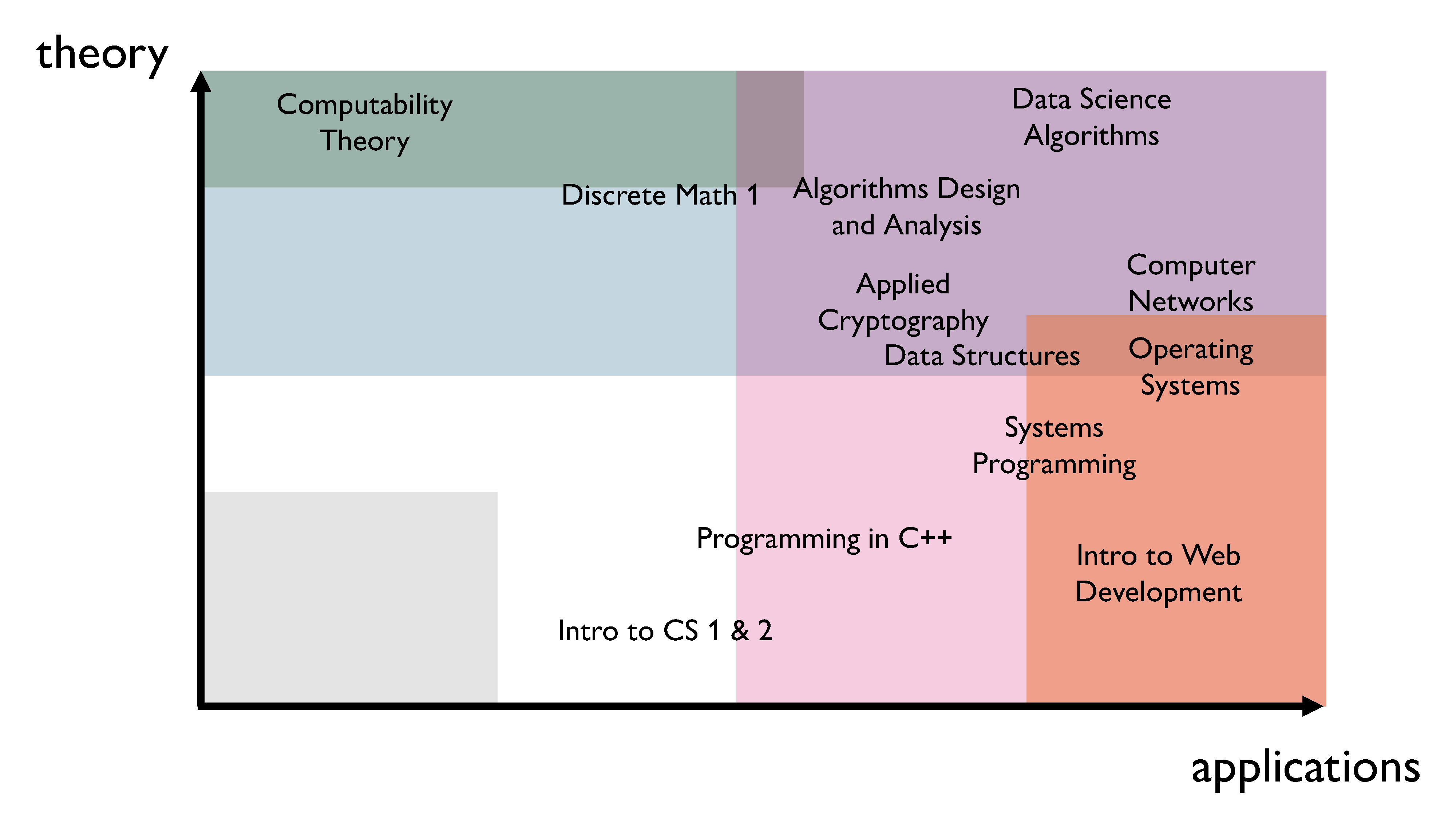
You should take this chart with a grain of salt – it’s really just my opinion. But as we can see, computer science degrees are very applied. However, as we get further into the degree, the theoretical component also steadily increases. In a lot of cases, it’s very difficult to fully decouple theory from applications, and doing so can actually be a terrible idea.
My goal isn’t to convince you to become a theorist, and especially not a pure theorist. There are other people out there with that goal: we call them math professors, and you should totally stay away from them. (Just kidding. Sort of.) But my goal is to help you understand why our degree forces us to take theory courses, especially the more math heavy courses, and also to maybe try to convince you that math can be interesting, because math courses aren’t always particularly convincing.
Disclaimers
I should probably mention that some of this is just my opinion, filtered through my experiences and worldview. That’s my disclaimer for the day: please take whatever I say with a grain of salt.
Also, I am not an expert. (Yet.)
WTF is “theory”?
So what do I mean when I say the word “theory”? I should probably get that out of the way first.
Dictionary definitions
Here’s a definition from Merriam Webster. I’m cherry-picking the points that I like and think are relevant here. (Here’s the full definition.) So we have:
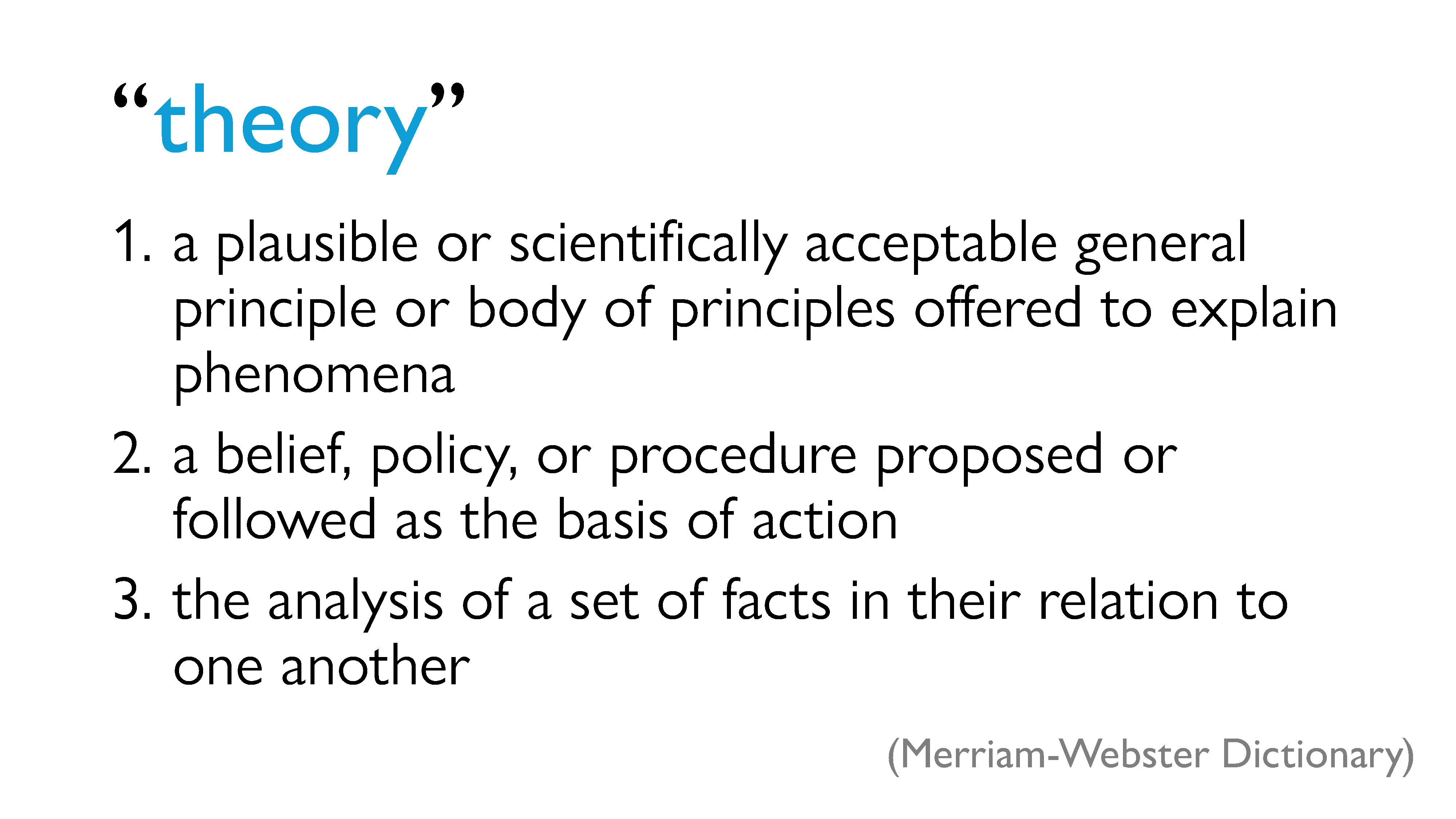
- a plausible or scientifically acceptable general principle or body of principles offered to explain phenomena
- a belief, policy, or procedure proposed or followed as the basis of action (here we can think of the scientific method as being a kind of theory, or a theoretical framework)
- the analysis of a set of facts in their relation to one another
I’m also going to show this other definition of theory from the Oxford Learner’s Dictionary. Again, I’m cherry-picking. (Full definition here.)
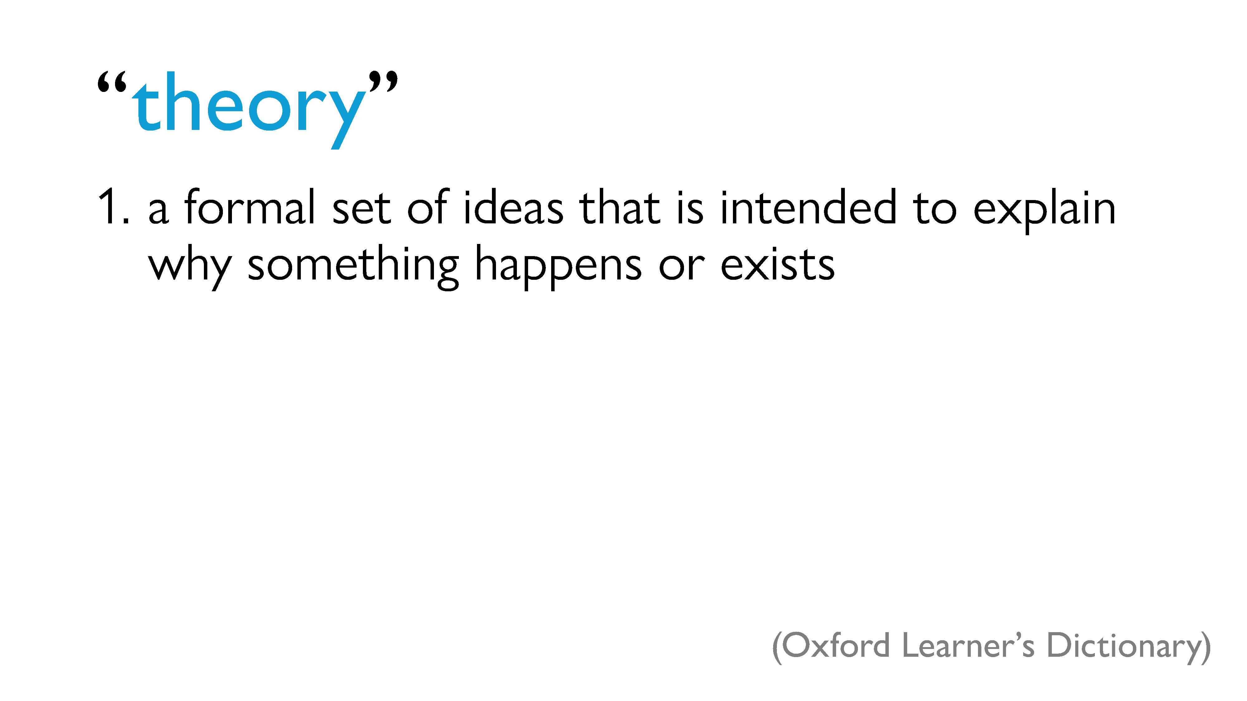
- a formal set of ideas that is intended to explain why something happens or exists
In summary, according to the two dictionaries, theory helps us understand where methods come from, why different phenomena occur, and how different ideas are related to each other. Theory is also a method for studying these ideas and phenomena.
That being said, I’d like to give my own slightly different definition, which I think will be more relevant for our purposes.
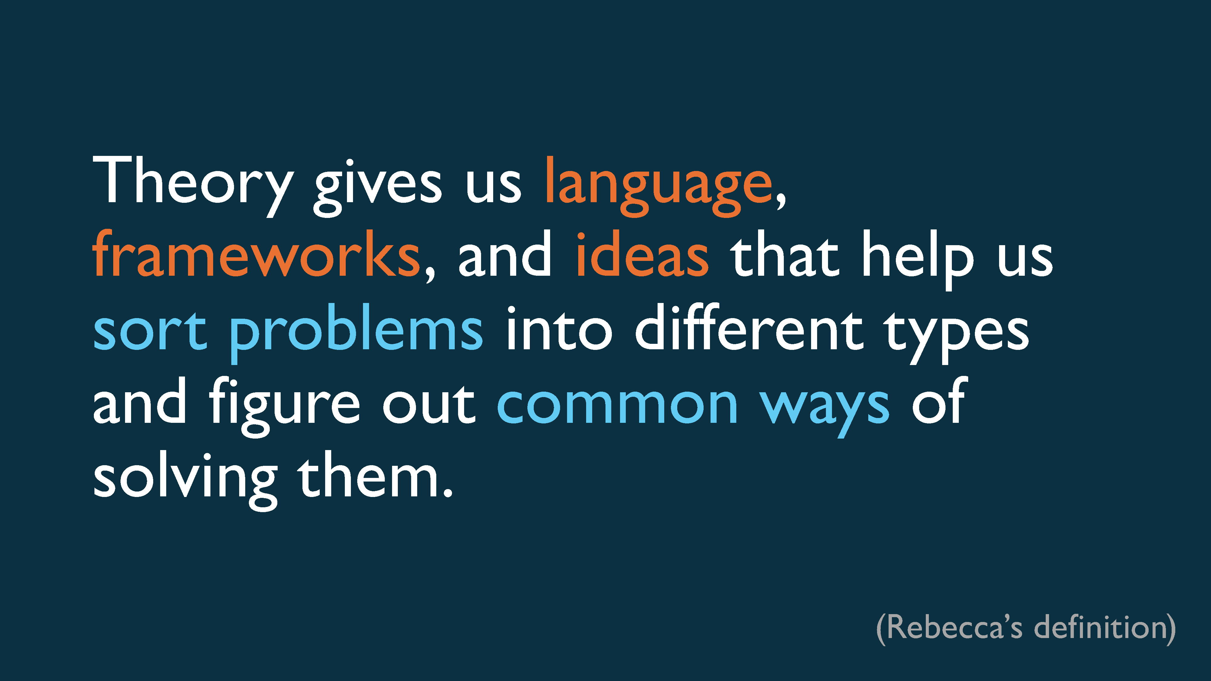
In the context of computer science, I like to think of theory as being something that gives us language for discussing different problems, frameworks for sorting them into different categories, and ideas for finding common ways of solving problems of a certain type.
Abstraction and Generalization
Two common tools that we often use in computer science are abstraction and generalization.
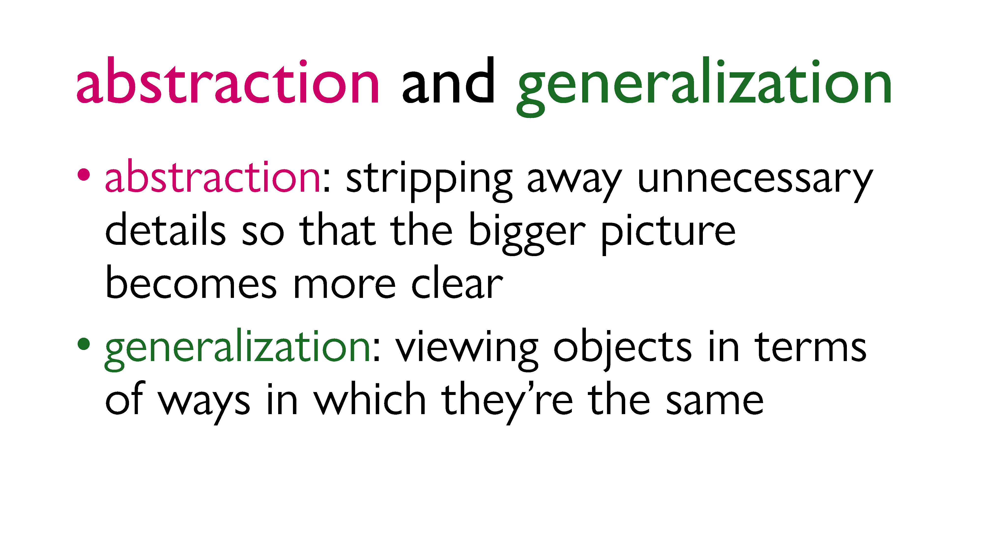
Abstraction is sort of like simplification: it’s stripping away unnecessary details so that the bigger picture becomes more clear. As we iteratively do this over time, the new abstraction might start to look really different from the thing we were originally describing, but the key is that the core idea is still captured – a person looking only at the abstraction should not feel like they’re missing crucial information.
Generalization is related, but slightly different: it allows us to classify larger and larger groups of objects by looking at ways in which they’re fundamentally the same. It can be an iterative process, in the sense that we can build classes that are contained within each other, and it’s not a unique process, in the sense that we can have classes that overlap with each other in different ways, and that there may be multiple ways to build classifications of the objects.
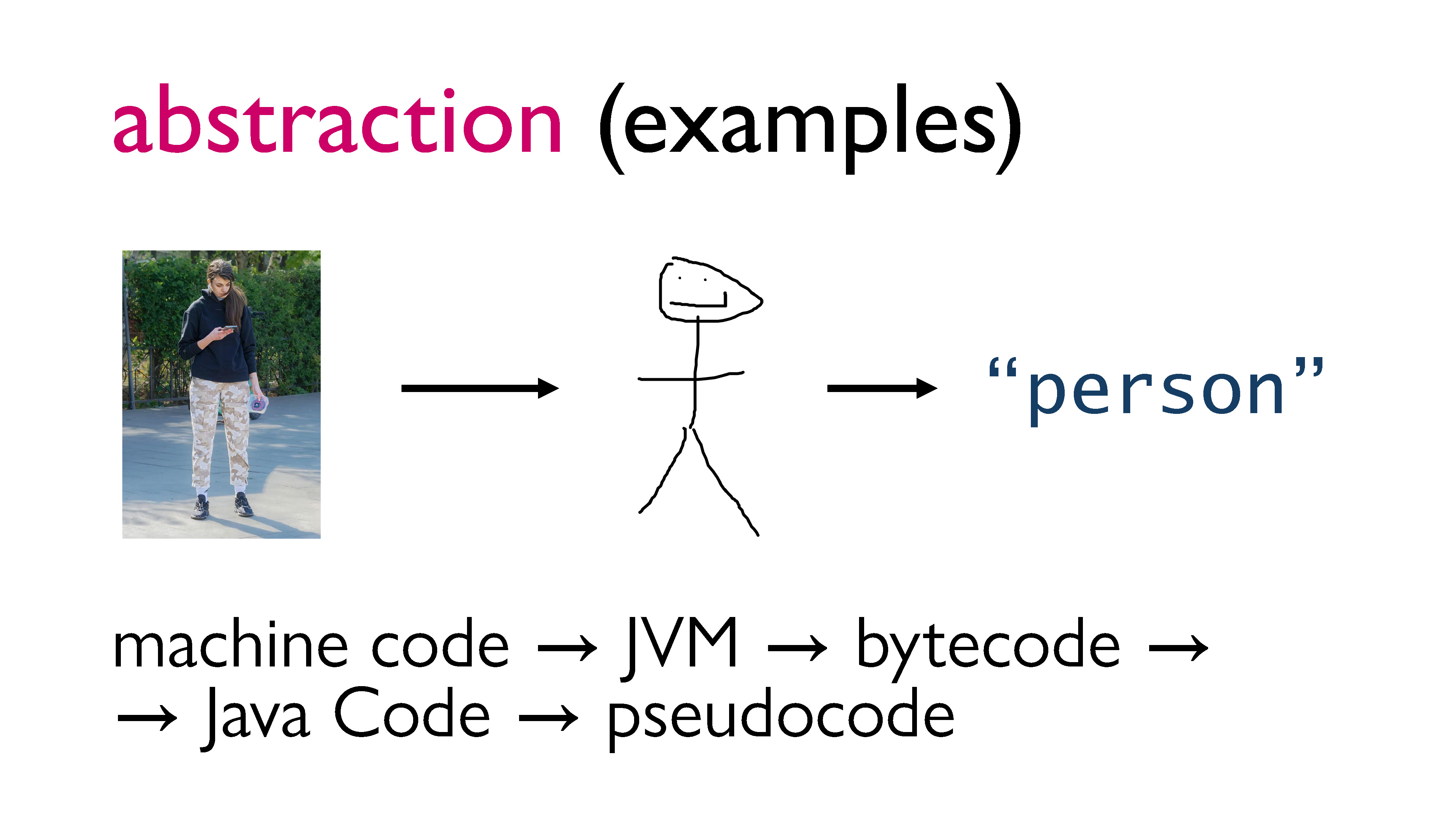
One example of abstraction is the evolution of language. We went from actually drawing things when we wanted to convey them, to using pictograms, to writing words that don’t even look like the original concept. So if I want you to think about the abstract idea of a person, I can show you a real person! But I could also show you a semi-realistic drawing, or a stick figure, or even just the word “person”, and you would still be able to hold the idea of a person in your head, even if the word “person” looks nothing like a human.
But we also do this sort of abstraction in programming all the time. You might have an idea for a program that you can describe using pseudocode, which is pretty abstract but captures the idea. Let’s say you hand off your pseudocode to a colleague to implement in Java. While your colleague is able to understand the program, they will need to add more details so that the computer can interpret it. If they want to then run the program, they will have to compile it first. The compiler will convert the program to bytecode, which will have more specific instructions for the Java Virtual Machine (JVM). When the bytecode is run on the JVM, it will be interpreted into machine code, which will have hardware dependent instructions. And as the code gets executed on the machine, it’ll go down the ladder of abstraction until it hits the level of logic gates that are being turned on and off.
As the original writer of the pseudocode, you don’t need to understand bytecode or machine code or logic gates. You probably don’t even need to know how to write code in Java! This is the beauty of abstraction.
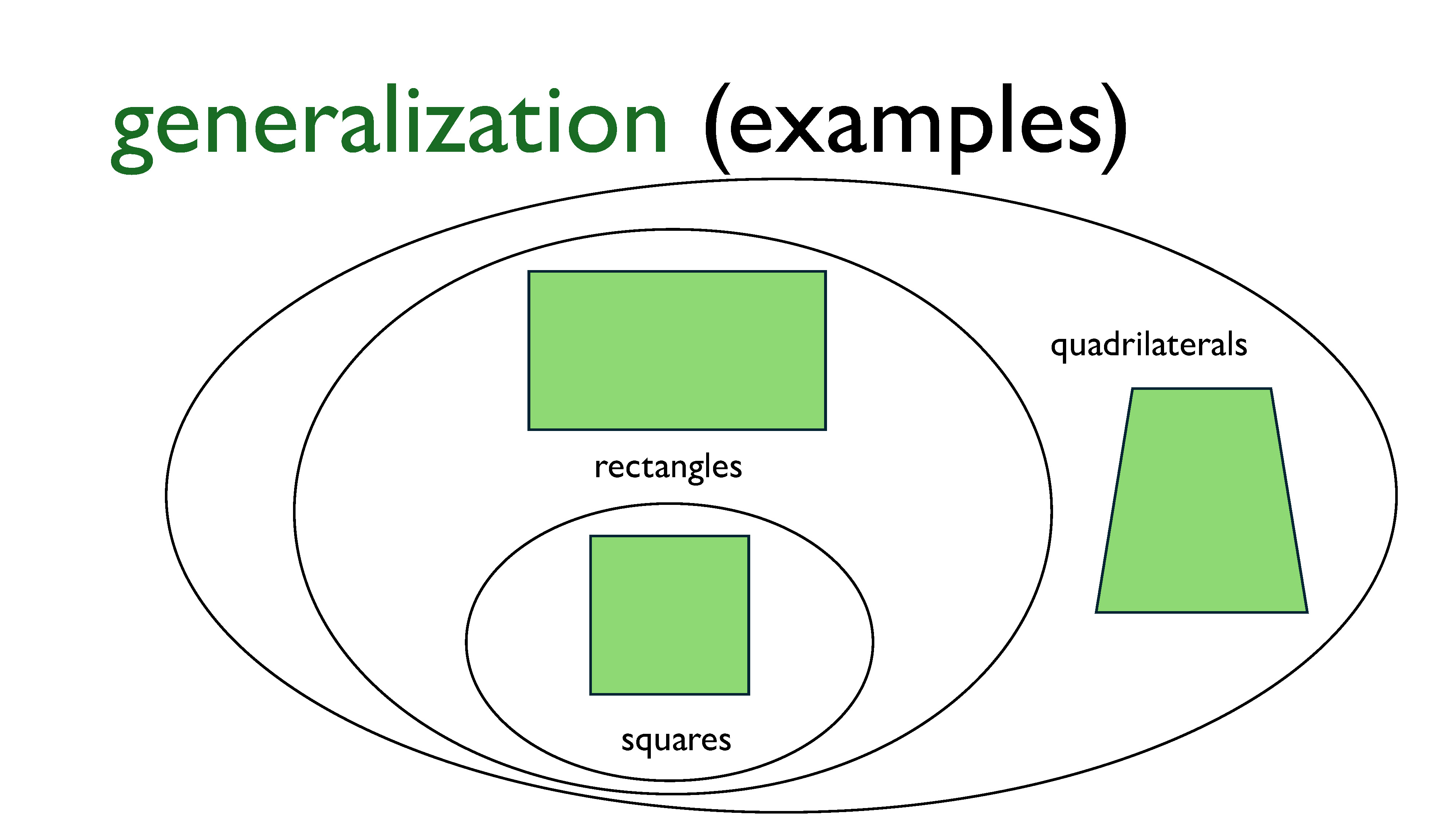
An example of generalization is this idea of classifying polygons. One way to classify them is based on the number of sides they have, the lengths of the sides, and their angles. As we can see in the slide, a square is a rectangle, which is a quadrilateral. We could extend this more: squares and rectangles are both trapezoids, and then we could have trapezoids that don’t have any symmetry, and lastly, quadrilaterals.
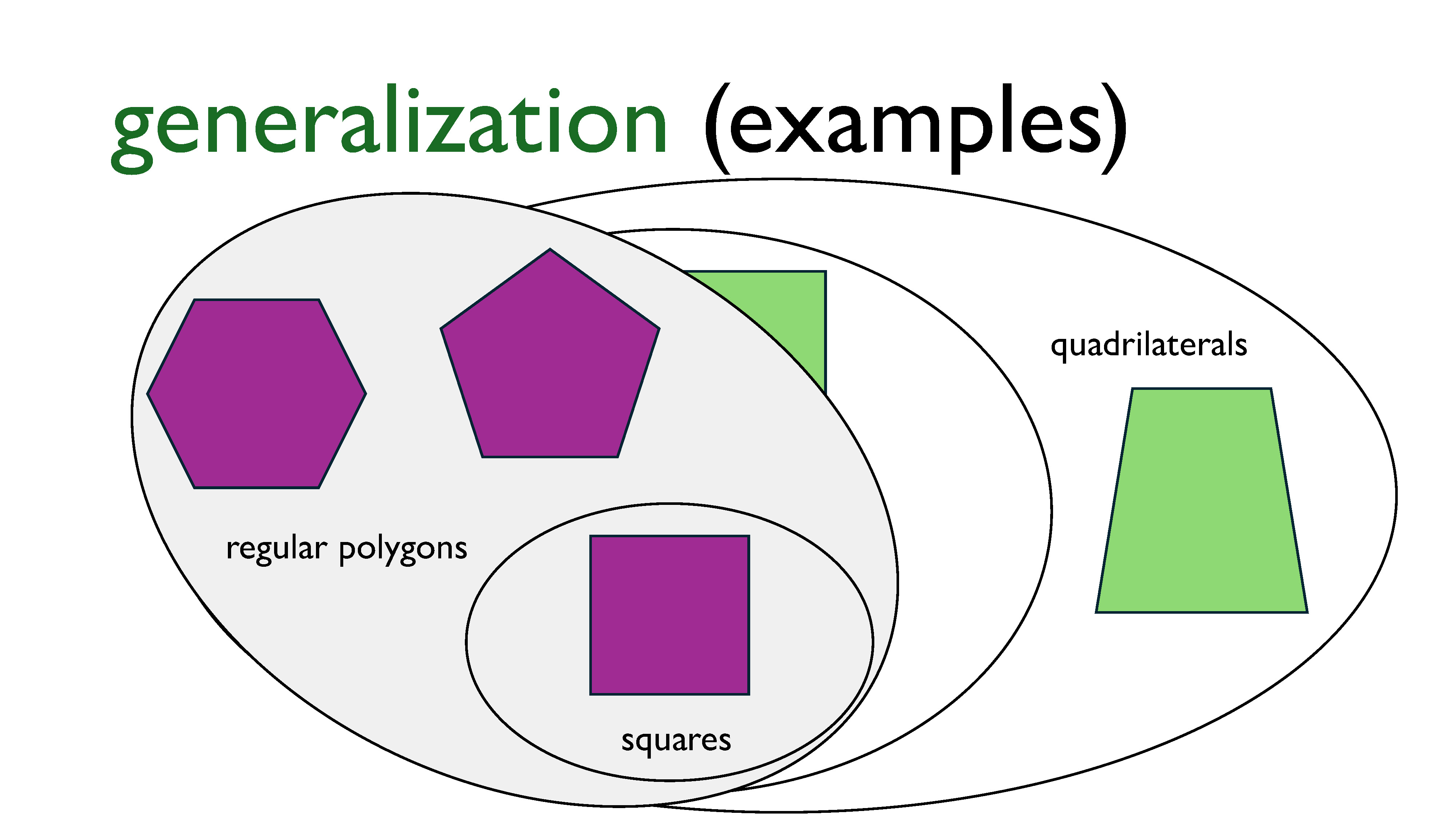
But squares are also regular polygons! So another way of classifying shapes might be to more coarsely separate them into regular polygons and irregular polygons, or even have some sort of category for polygons that have some symmetry to them but aren’t quite regular.
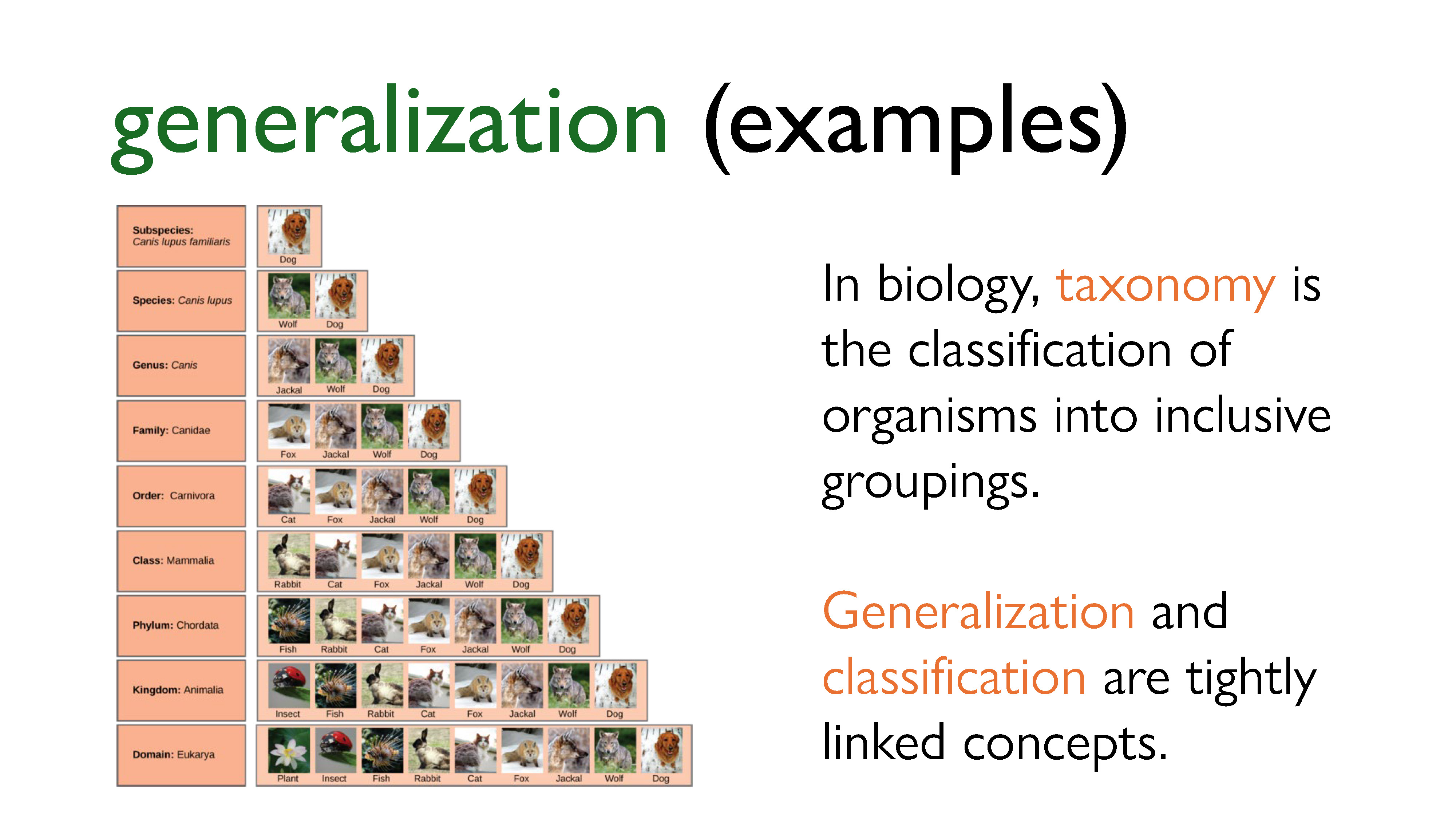
We also see the idea of generalization a lot in biology, especially when it comes to classifications. Taxonomy is all about classifying species into hierarchical classes of groups with shared characteristics, using a defined and systematic process.
Theory \(\neq\) Math!
The last thing I want to say as part of this “defining theory” section is that contrary to popular opinion, mathematicians do not have a monopoly on theory. There are lots of ways to use theoretical tools and approaches without ever dealing with math, and lots of them are useful in computer science! Being able to break down and understand problems and ideas is a universally applicable skill that manifests itself in lots of different ways.
However, math is often useful in theoretical contexts, especially when the problems being tackled, or the questions being studied, are of a quantitative nature. This is because math is a very precise language for describing problems, and also abstracts away a lot of (at times irrelevant) qualitative details. This can be very helpful when trying to come up with generalized solutions to problems. But please do note that I never said mathematical language was clear. Contrary to what your math professors might tell you, mathematical language is often very unclear and can be difficult. But it is precise, and that precision can be key.
So where are we going with this? I know I just said that theory is not synonymous with math, but as it happens, I am going to be talking about math today. That’s just because the problem I’ve been studying for the past several months is very mathematical in nature, and I want to use it as a case study. I want to provide an example of how the ideas I’ve just discussed might be actually used in computer science, and give you an idea of why math-adjacent courses (like a course in discrete math, or a course in algorithms, for instance) shouldn’t be written off as a waste of time.
For the rest of this talk, I’m going to go up and down the ladder of abstraction to show you why we do theory, and concretely show you how it is useful.
First, we’re going to look at some real-world problems. We’re going to precisely describe these problems using math, and we’re going to look at some solutions for these problems. Then, we’re going to see how generalizing these solutions can give us solutions to some related problems for free.
And that, right there, is the power of theory.
Part 2: Real-World Problems and a Crash Course to Graph Theory
Some interesting “real-world” problems
In the first part of this talk, I made the case that theory is useful because it allows us to find (or at the very least, have the correct toolkit and language to explore) solutions to real-world problems. In this part, we are going to look at some examples of such problems and develop mathematical language to be able to discuss them more abstractly.
I’ve put the term “real-world” in quotes in the title, because I’m going to be talking about these problems in a lot of generality. However, I want to stress that specific instances of these problems are actually relevant in industry, and I think it’ll be easy to see why once I start talking about them.
I also want to want to point out that by giving general definitions of problems with a lot of details left out for clarity, we are already taking a first step onto the ladder of abstraction.
Community detection
The first problem we’re going to look at is what we call “community detection”, applied to the internet in this case. The idea is that we’re trying to group websites and pages into categories without actually reading every web page, because that would be impossible. So, how else can we detect groups of web pages that are related to each other? And how can we find the most “authoritative” or “important” web pages in each group?
This problem is a little bit less relevant now than it used to be, because the distribution of information on the internet has changed drastically over the years. The first papers about community detection were written in the 90s, when the Internet was still a collection of individual web pages, with links between them. At the time, most people on the internet maintained their own websites and primarily published content on their own sites. Nowadays, most of the Internet seems to exist on a very small group of social media platforms, which is where most content is being circulated. (See the idea of the internet consisting of five websites, each consisting of the other four. Tom Eastman said it first; Cory Doctorow popularized it.)
That being said, there are still billions of pages on the internet. If you’re a search engine, like Google, or an advertiser, like Google, this problem is probably relevant to you. (Though, if you’re as big as Google, you’re likely solving it using much more sophisticated techniques than what we’ll see here.)
Topic clustering
The next problem is topic clustering. Let’s say you’re a content platform, like YouTube, and there’s all this user generated content flooding your platform. How do you figure out which groups of content are similar or related enough to appeal to similar groups of people? Also, how do you figure out which groups of content are the most likely to be popular?
This problem is also known as large near-clique extraction, which is terminology that comes from graph theory. I’ll explain this a little bit more later on.
Correlation mining
Let’s say you’re an investment firm, and you’re trying to predict trends in the market so that you can make money for your clients. There are all sorts of assets you could be investing in or betting against, and many of them are interlinked with other assets. You may want to figure out which groups of assets are the most influential in the market. So how are the assets grouped? How do the groups relate to each other? Which groups of assets have the most influence on other groups?
These sorts of questions are an example of something called correlation mining – finding and analyzing relationships (“correlations”) between objects to determine which objects are the “most important.”
There are analogs of this question in genetics (for example, when trying to determine which genes will be expressed), in neuroscience, in spam detection, and so on.
How do we solve these problems?
I hope I’ve managed to convince you that these problems are important, or, at a minimum, that at least some of them are worth spending time to think about. At this point, the question becomes, how do we solve these problems?
It is also important that we figure out a way to solve these problems efficiently, that is, within a reasonable amount of time. YouTube can’t afford to wait around for an algorithm that takes years (or some other ridiculous amount of time) to finish running, because YouTube is out here trying to make money! Inefficient algorithms aren’t great in most real-world contexts because they take forever to terminate (if ever) and bleed money and resources.
If you’ve been looking closely, you may have noticed that these all kind of sound like the same problem. Or at the very least, they all sound like similar problems. In fact, if we abstract away some details, these can all be considered instances of the densest subgraph problem.
Graph theory: a crash course
Before I can talk about the densest subgraph problem (or DSP for short), I have to give you a crash course on graph theory. The language of graph theory is the abstraction that will allow us to describe a generalized solution for the previous problems we just looked at. In fact, graphs are so useful as a tool for representing problems in computer science that they’re impossible to avoid in a CS degree.
If you’ve already been introduced to graph theory, feel free to skip this section.
A graph is a way of representing pairwise relationships between objects.
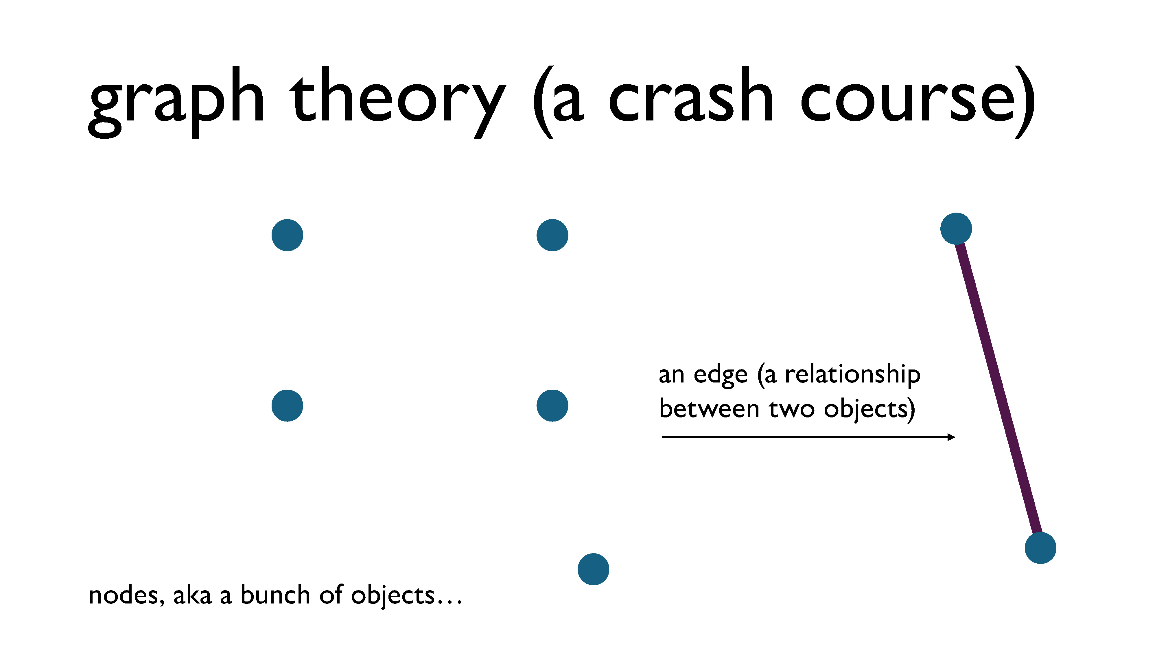
We represent the objects using what we call vertices (also called nodes) and we put an edge between two vertices if the objects are related. (I tend to use the word “node” when talking abstractly about the objects and the word “vertex” when discussing a drawing of a graph – that’s just a habit that I have – but they’re pretty much interchangeable words and they are used interchangeably.)
A pairwise relationship we often use as an example in graph theory is friendship: our objects are people, and we put an edge between two people if they’re friends. This, for example, is how relationships are described on Facebook.
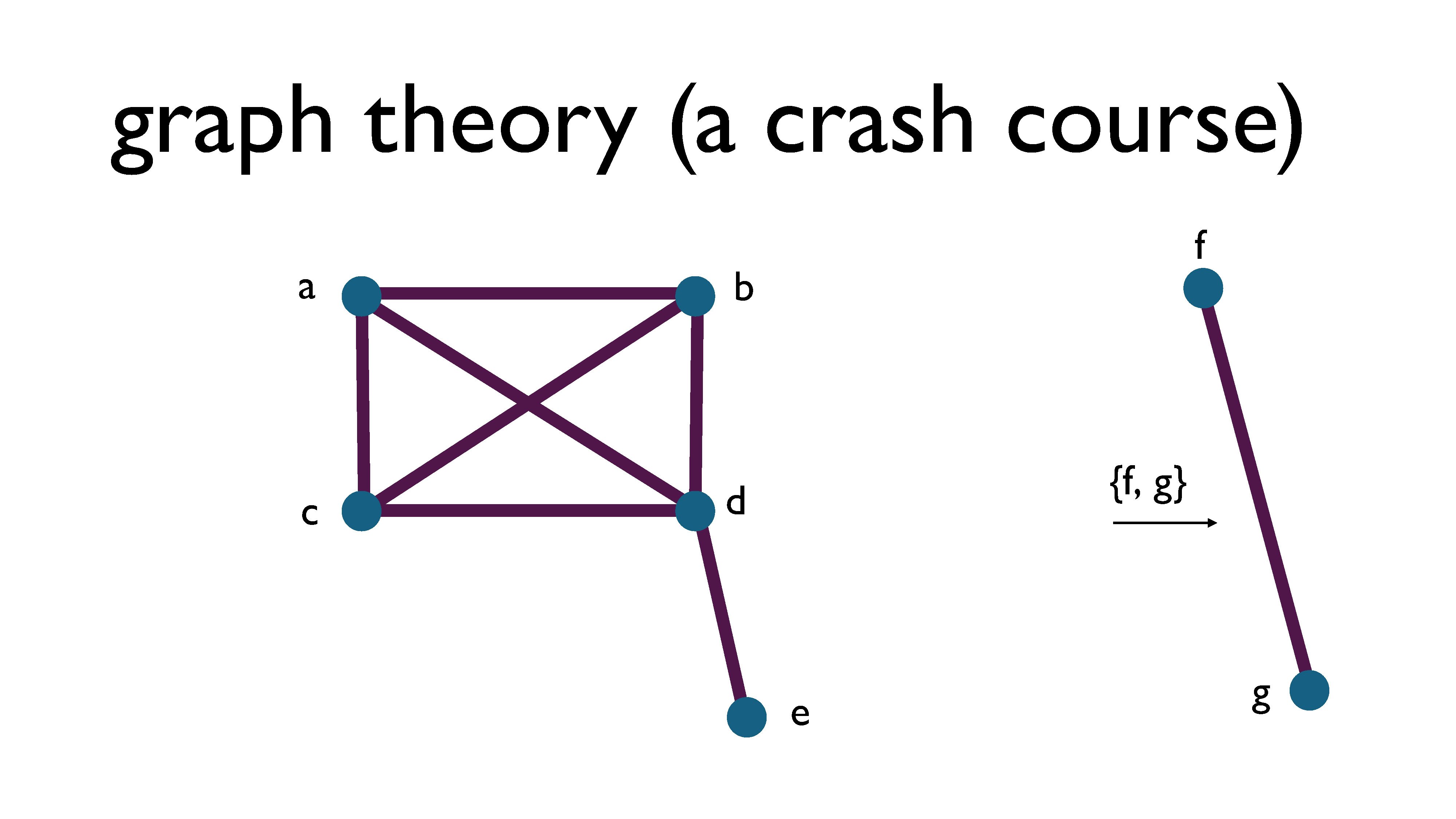
Here’s a graph that’s a little bit more interesting than the previous graph. Notice how I’ve labelled the vertices – we often do this to make talking about the graph a little bit easier.
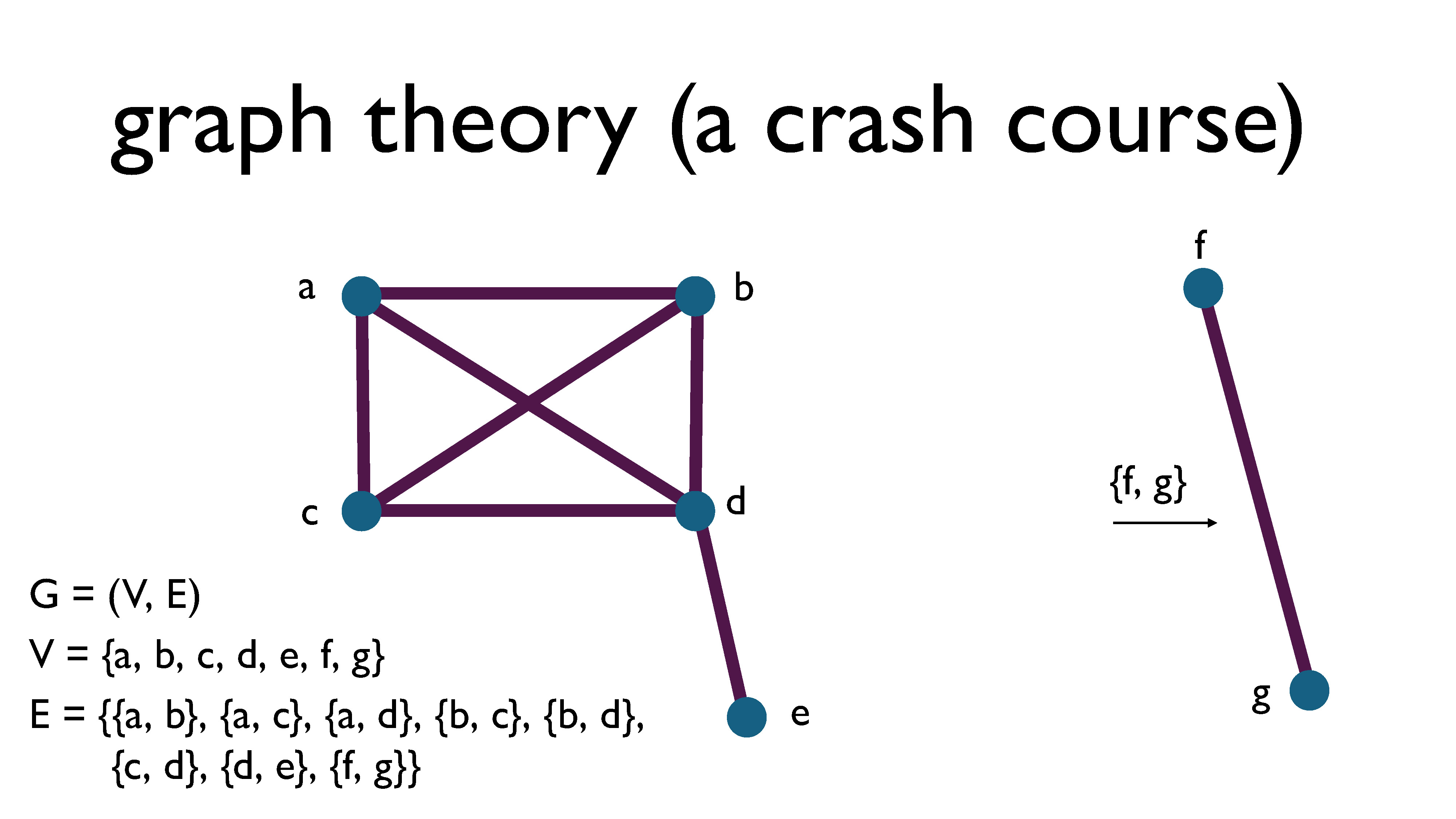
Formally, a graph, denoted \(G\), is defined as a pair consisting of a set of vertices \(V\) and a set of edges \(E\), where each edge is a two-element subset of the vertices. For example, in the picture above, the edge between f and g is represented by the subset \(\\{f, g \\}\). This is called an undirected graph.
(You can also look into hypergraphs, which are generalizations of graphs. I previously wrote a primer on hypergraph theory, which you can find here.)
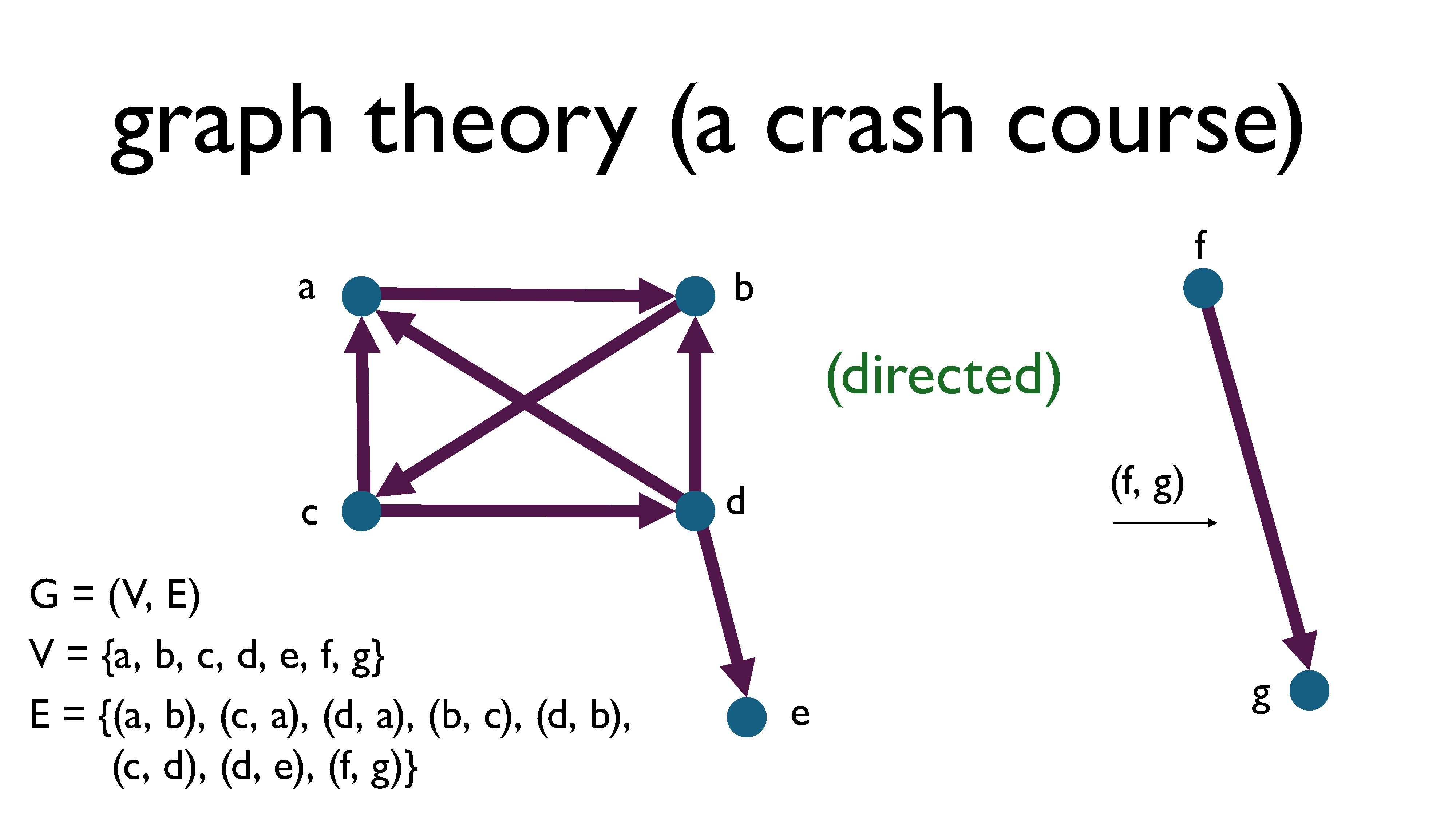
There are also directed graphs (sometimes called digraphs), where edges are ordered pairs, meaning that each relationship is one sided. For example, following someone on Twitter is a one-sided pairwise relationship: if I follow you on Twitter, that does not imply that you will follow me back. This is different from friendship on Facebook, where if I’m friends with you, that implies that you are also friends with me. An edge \((a, b)\) in a directed graph is represented by an arrow going from vertex \(a\) to vertex \(b,\) with the arrowhead pointing at \(b\).
I only mentioned directed graphs for completeness, since we’re mostly going to ignore those in this presentation. Whenever the word graph is used without qualification, it’s generally understood to be referring to an undirected graph.
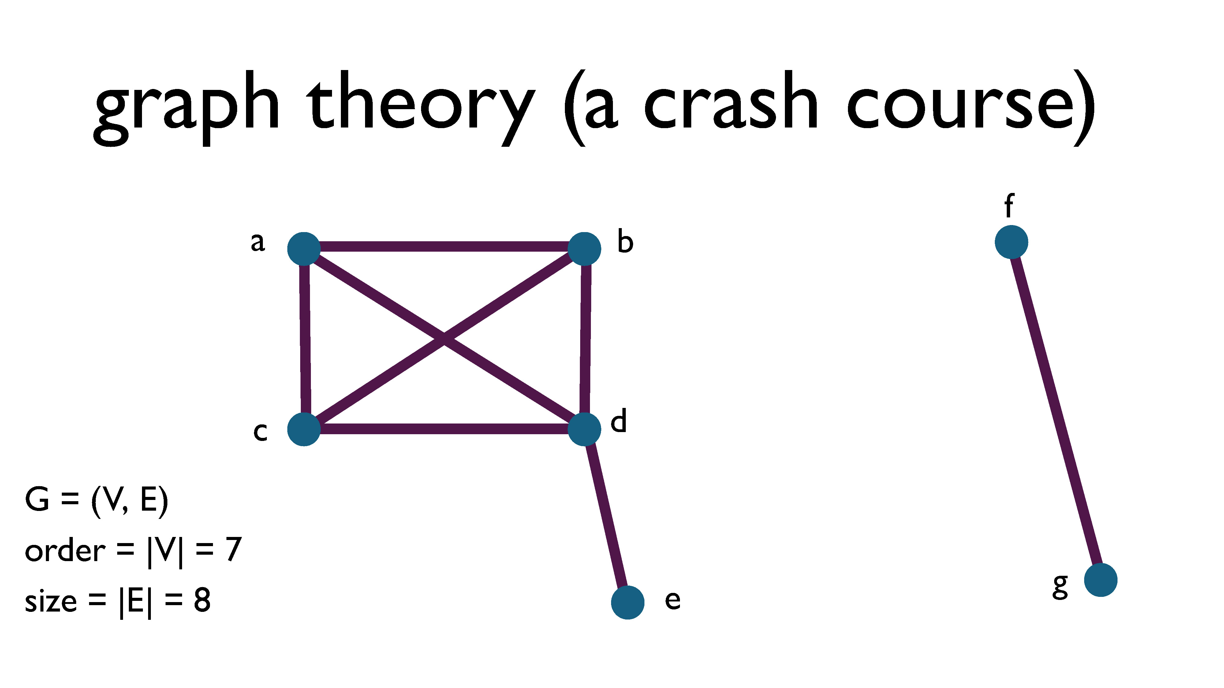
The order of a graph is the number of vertices in the graph, and the size of a graph is the number of edges it contains.
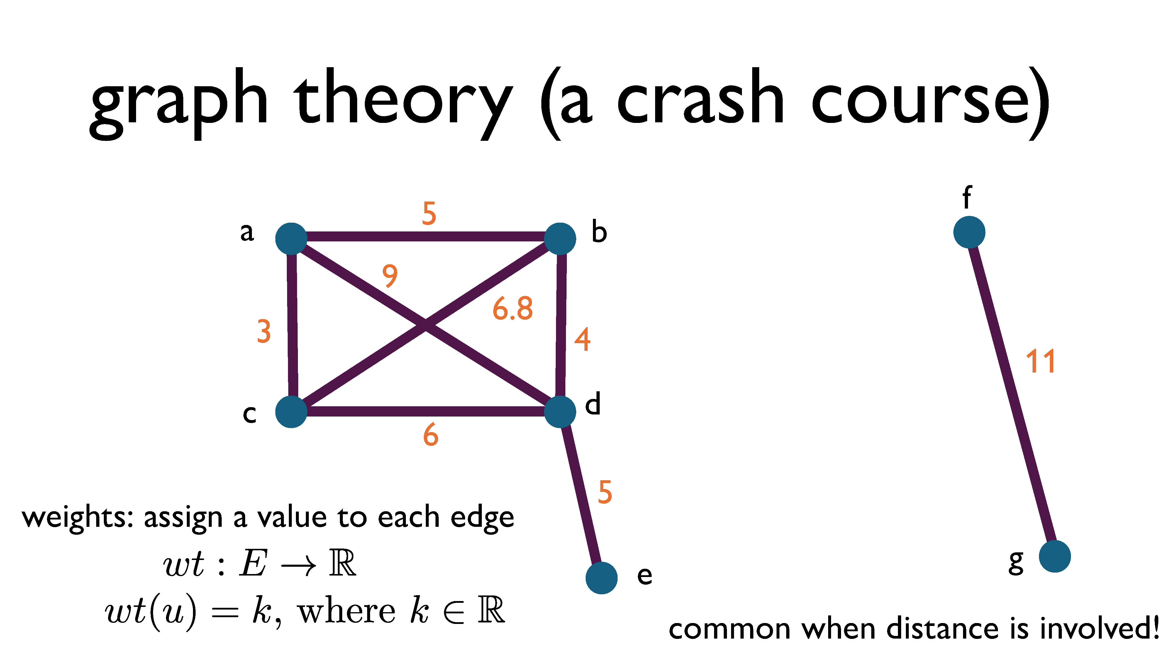
A graph can be weighted. This means that every edge is assigned a number, which typically has an actual meaning associated with it. This is really common when we’re talking about maps and geometry or space related problems. Then, nodes are locations, edges are roads, and weights are the distance between two locations. You can also have negative weights on a graph (but we’re not going to go there in this presentation).
Formally, a weighted graph is a graph \(G = (V, E)\) together with a weight function \(wt: E \rightarrow \mathbb{R}\) that maps every edge to a real number.
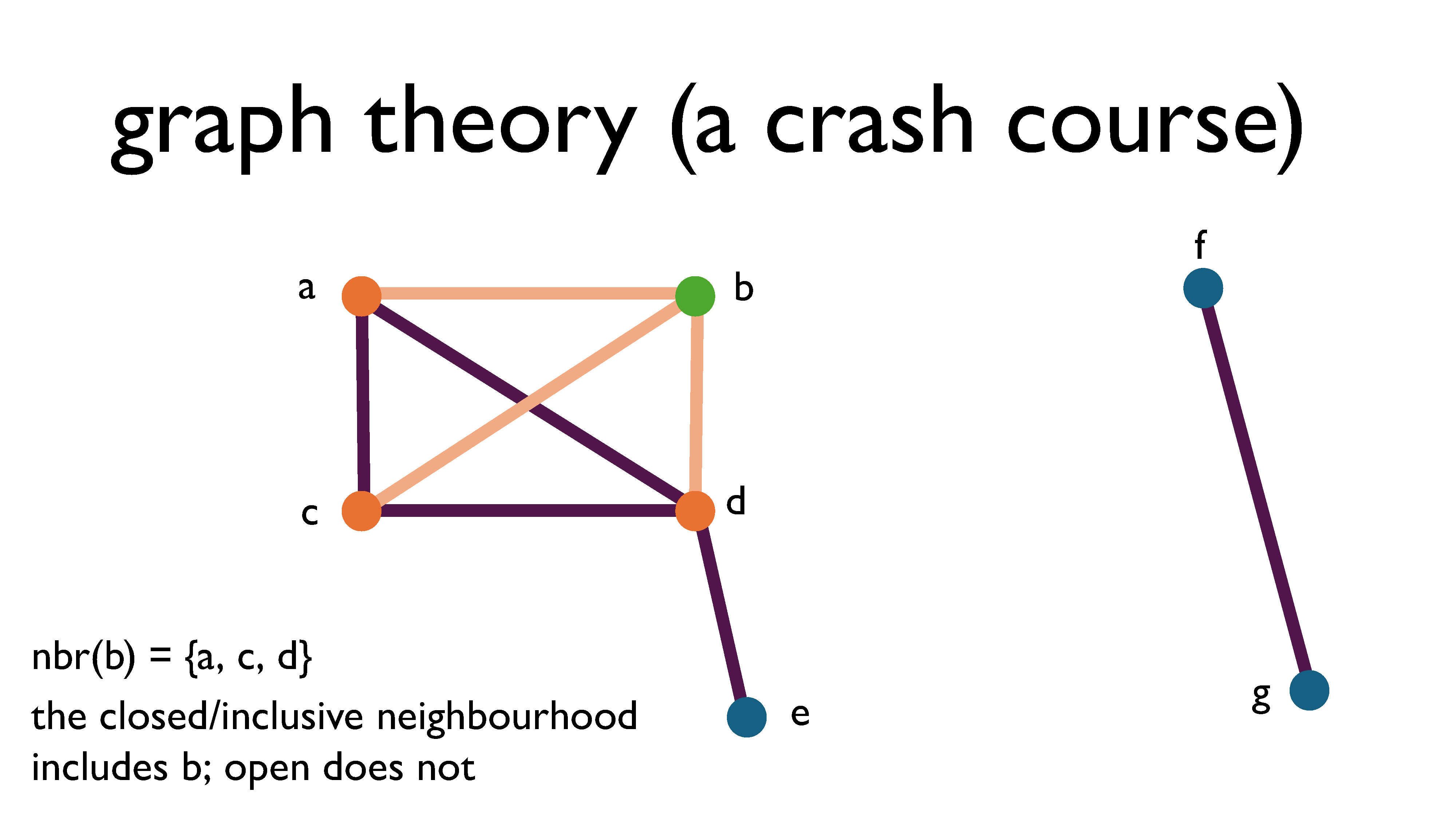
The neighbourhood of a vertex is the set of vertices it shares edges with. When we say the word neighbourhood on its own, we usually mean the open neighbourhood, which is just the vertices on the other end of the edges. The closed (or sometime you’ll hear “inclusive”) neighbourhood includes the original vertex.
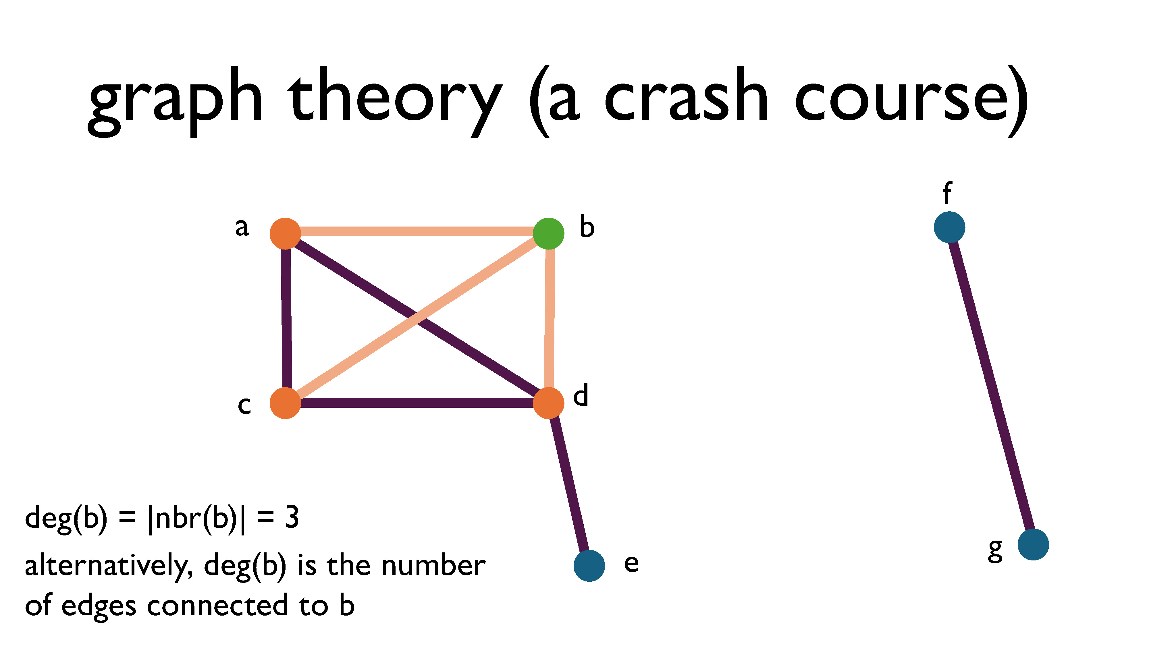
The degree of a vertex is the size of its open neighbourhood, aka the number of edges connected to it. For directed graphs, we instead have the concept of in-degrees and outdegrees. The in-degree of a vertex is the number of edges pointing into the vertex, and the out-degree of a vertex is the number of edges pointing away from the vertex.
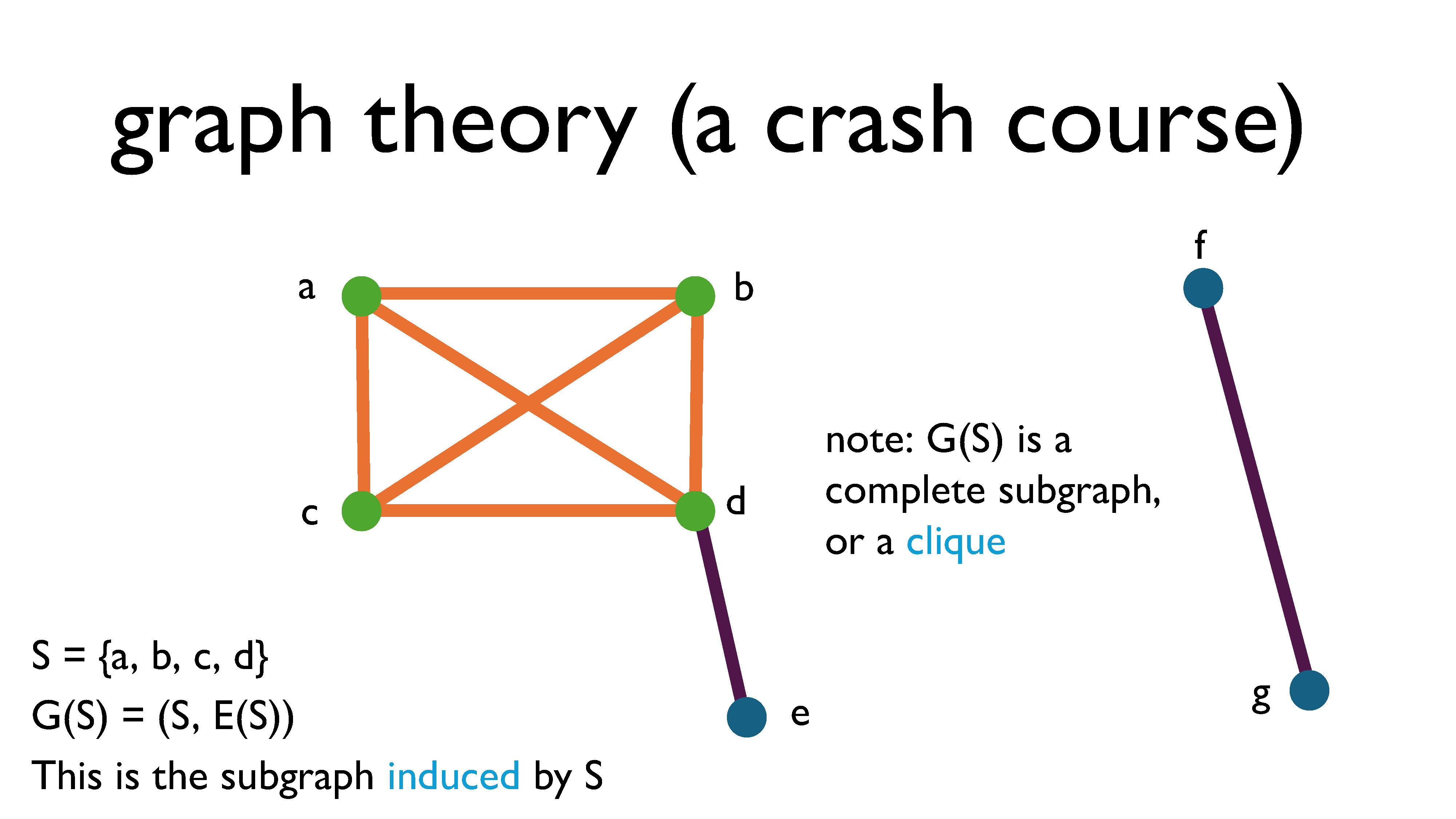
A subgraph is a graph that you get by choosing some of the nodes and some of the edges. If you pick some subset of vertices (let’s call it \(S\)), and force all of the edges with both endpoints in \(S\) to be part of the subgraph, we call that the subgraph induced by \(S\) and denote it \(G[S]\) (this is the orange and green part of the graph shown above). We denote the edge set of \(G[S]\) by \(E(S)\).
A graph is called complete if all of its vertices shares edges with every vertex. The complete graph on \(n\) vertices is denoted \(K_n.\) A subgraph is called a clique if it’s a complete subgraph.
Okay, so maybe that was a lot to digest, especially if you’ve never seen graph theory. However, this was really just meant to be a crash course to introduce basic ideas and definitions. But now we’re equipped to revisit the problems we looked at earlier to see how they’re all connected!
Back to the real-world problems
Let’s go back to our original real-world problems and connect them to graphs.
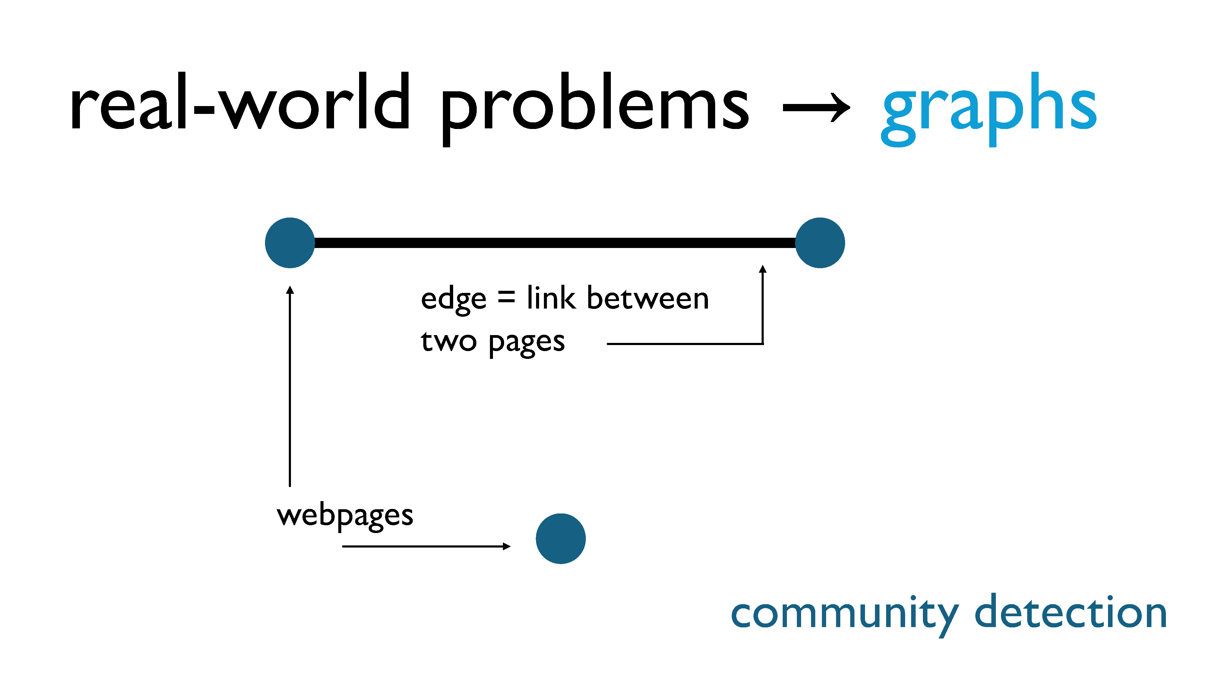
For community detection, the nodes are webpages, and there is an edge between two pages if one page links to the other.
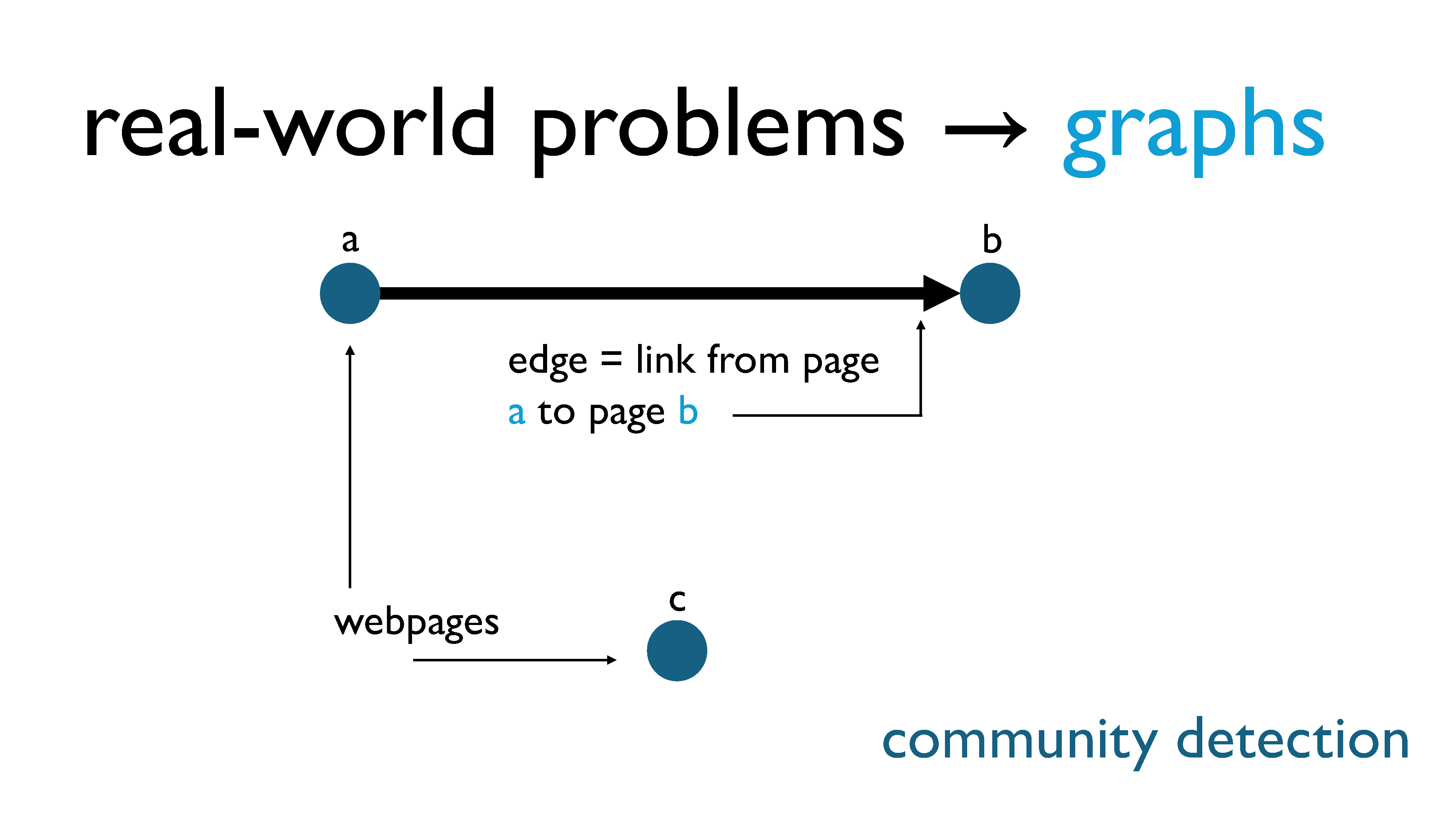
Technically, this should be a directed graph… but we’re just going to ignore that detail.
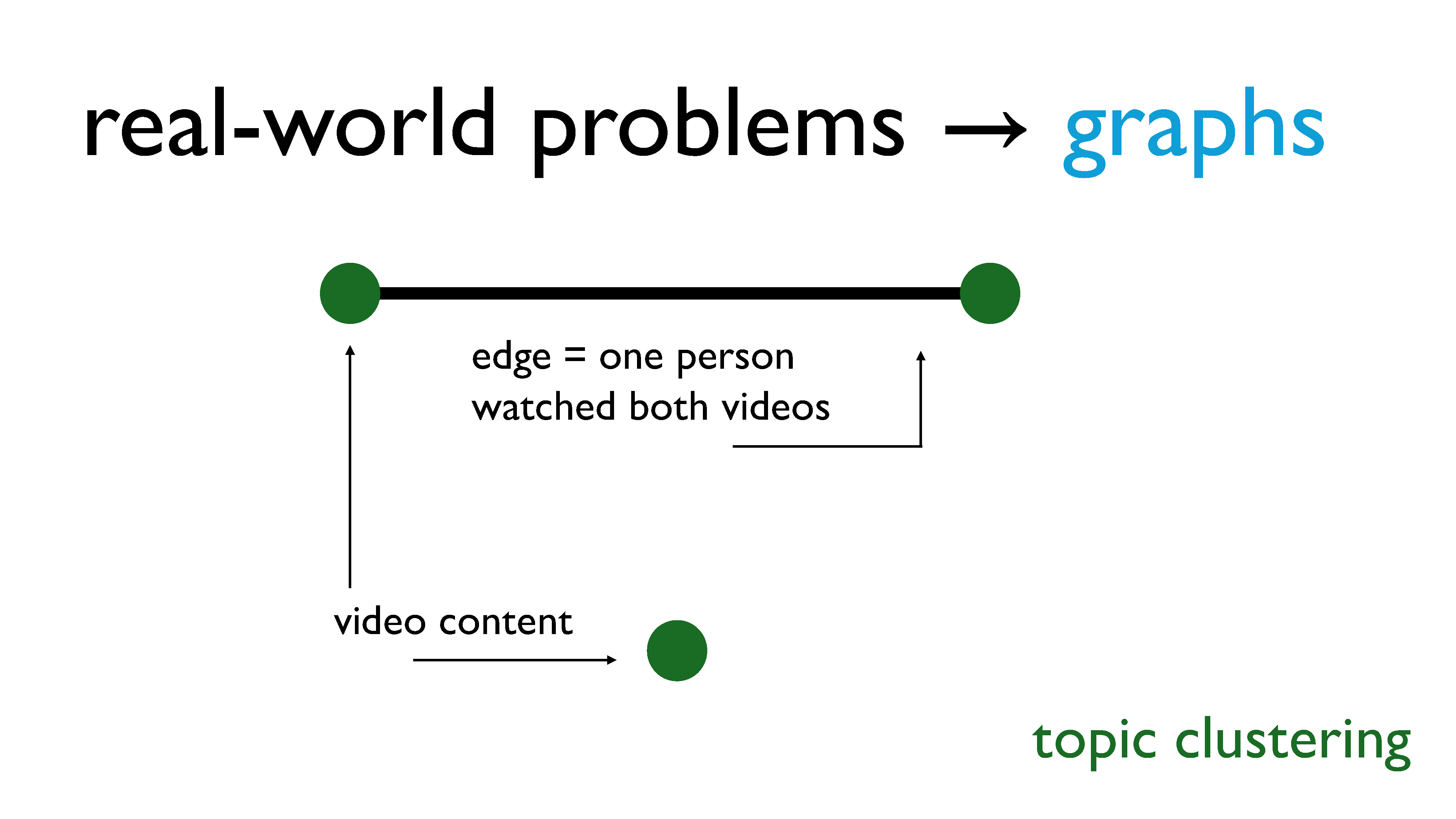
For topic clustering, our nodes are video content, and we put an edge between the two nodes if at least one person has watched both pieces of content.
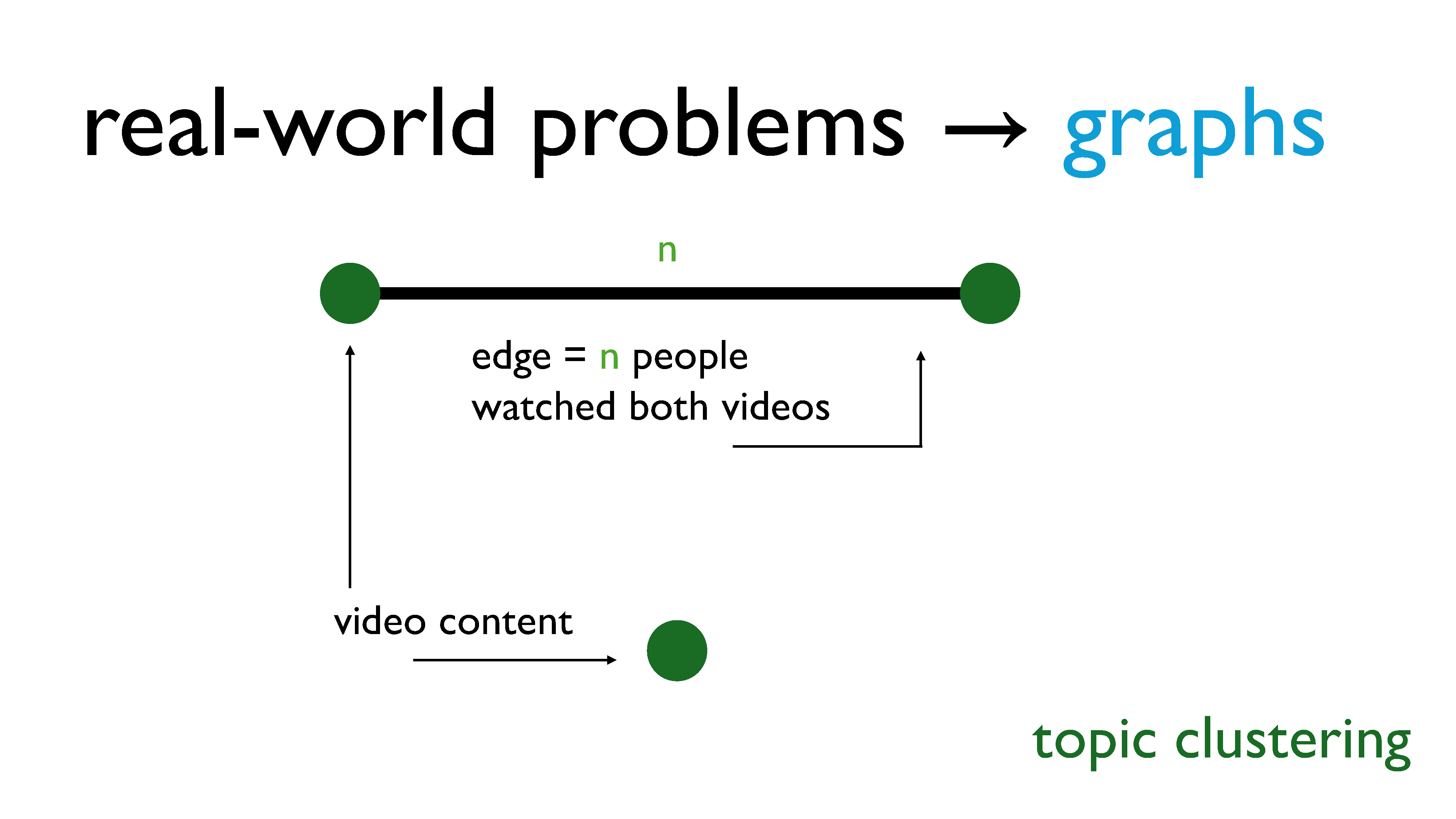
Technically, this is a weighted graph, where the weights are the number of people who have watched both videos. But again, we’re just going to ignore that detail.
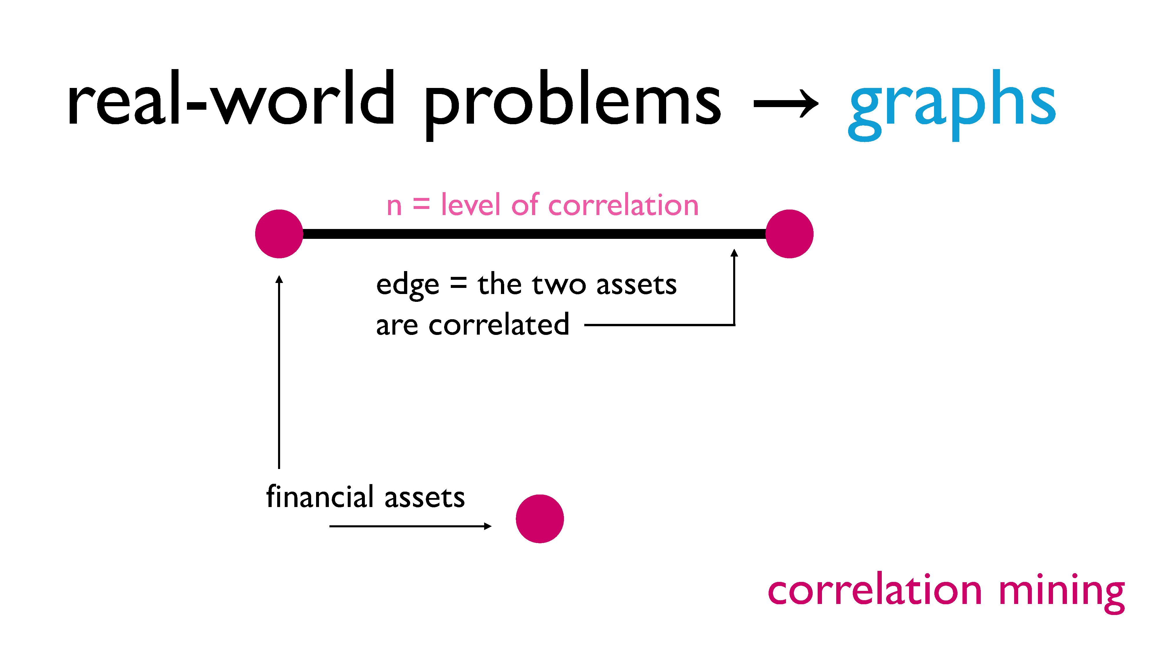
For financial correlation mining, our nodes are assets, and we put an edge between two nodes if the two assets are correlated – that is, if they have a direct influence on each other.
Now we know we can represent all of our previous problems as graphs!
To conclude this section, let’s revisit the notion of large near-clique extraction. We just learned that a clique is a subgraph in which each vertex shares an edge with every other vertex in the subgraph. A near-clique, then, is a subgraph in which each vertex shares an edge with most of the other vertices in the subgraph.
What these problems all have in common is that finding the largest near-clique is a pretty good way of identifying the “most important” objects. We’ll be identifying how exactly we can find such a subgraph when we look at the densest subgraph problem more closely in Part 3.
Part 3: The Densest Subgraph Problem, Peeling, and Iterative Peeling Algorithms
Abstraction: The Densest Subgraph Problem (DSP)
In Part 2 of this talk, we gave a crash course to graph theory and showed how we can use it to view some real-world problems as instances of the densest subgraph problem (DSP). But what exactly is the DSP?
If you’ve studied graph theory, you may have heard of something called the Maximum Clique Problem. The goal of the max clique problem is to find the largest complete subgraph in a graph. If we consider our vertices to be people, and edges to represent a friendship relationship between two people, in the max clique problem we are trying to find the largest friend group in a community. This is a famously difficult problem – it is NP-Hard, meaning that we strongly believe that creating an algorithm that does this efficiently is impossible.
The DSP can be viewed as a loose extension of the max clique problem: in this case, we are trying to find the subgraph with the highest average degree. Going back to our example, this means we want a group of people where on average, each person is friends with a large number of people. You could also see it as the group where “the most people know each other”, or as the group that maximizes the ratio of friendships to people.
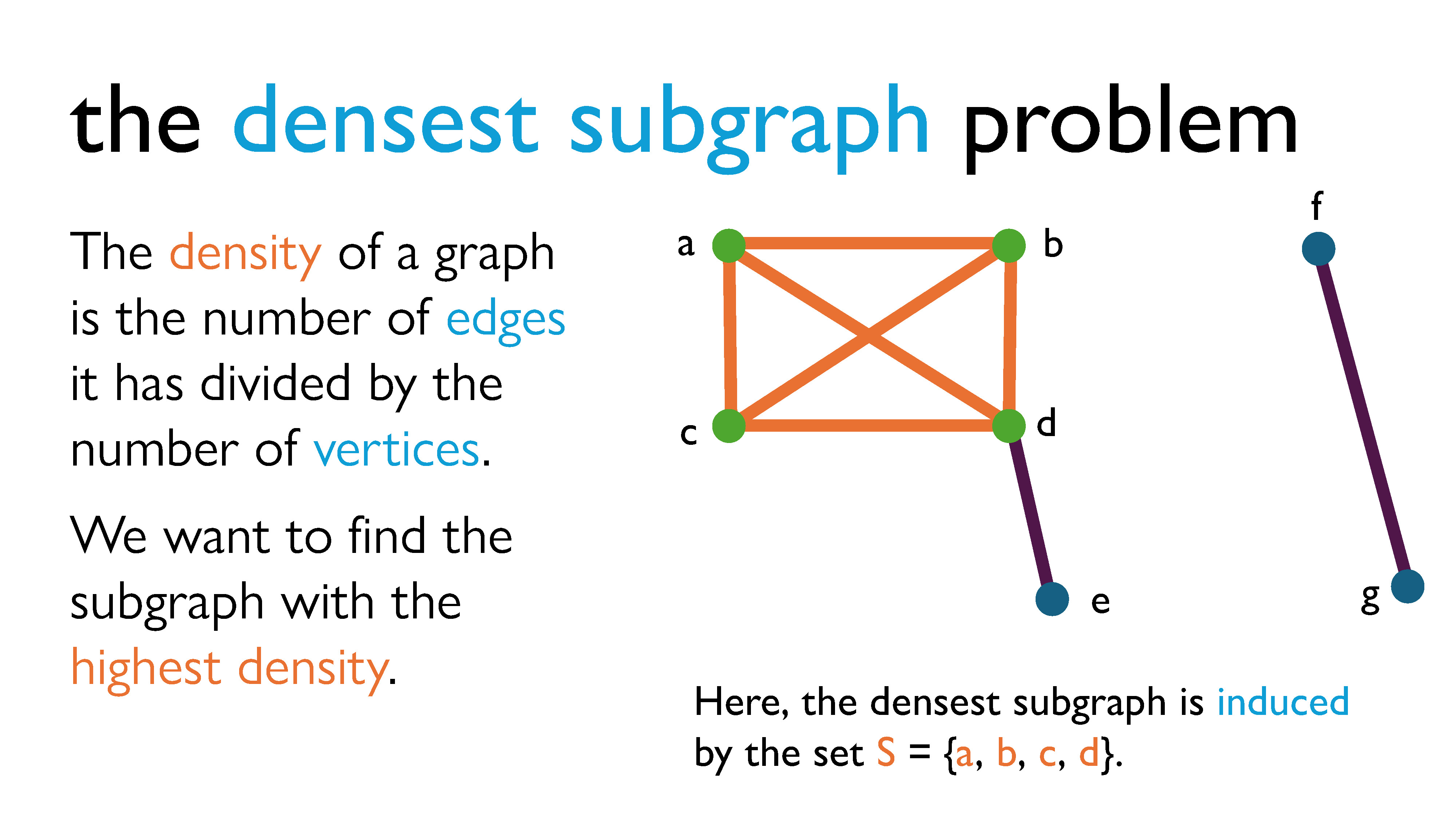
If we go back to looking at graphs more concretely, the density of a graph is usually defined by the number of edges it has divided by the number of vertices it has, and when solving the DSP we try to find the subgraph with the highest density. The term “density” comes from the idea of finding a subgraph that maximizes some ratio with respect to the properties of the graph. Usually, that property is the ratio of edges to vertices (aka relationships to objects), and that’s typically what we refer to when we talk about the DSP. (It’s also what we will focus on for now.) However, I should probably note that there are many variants of the DSP, which use all sort of other types of density measures.
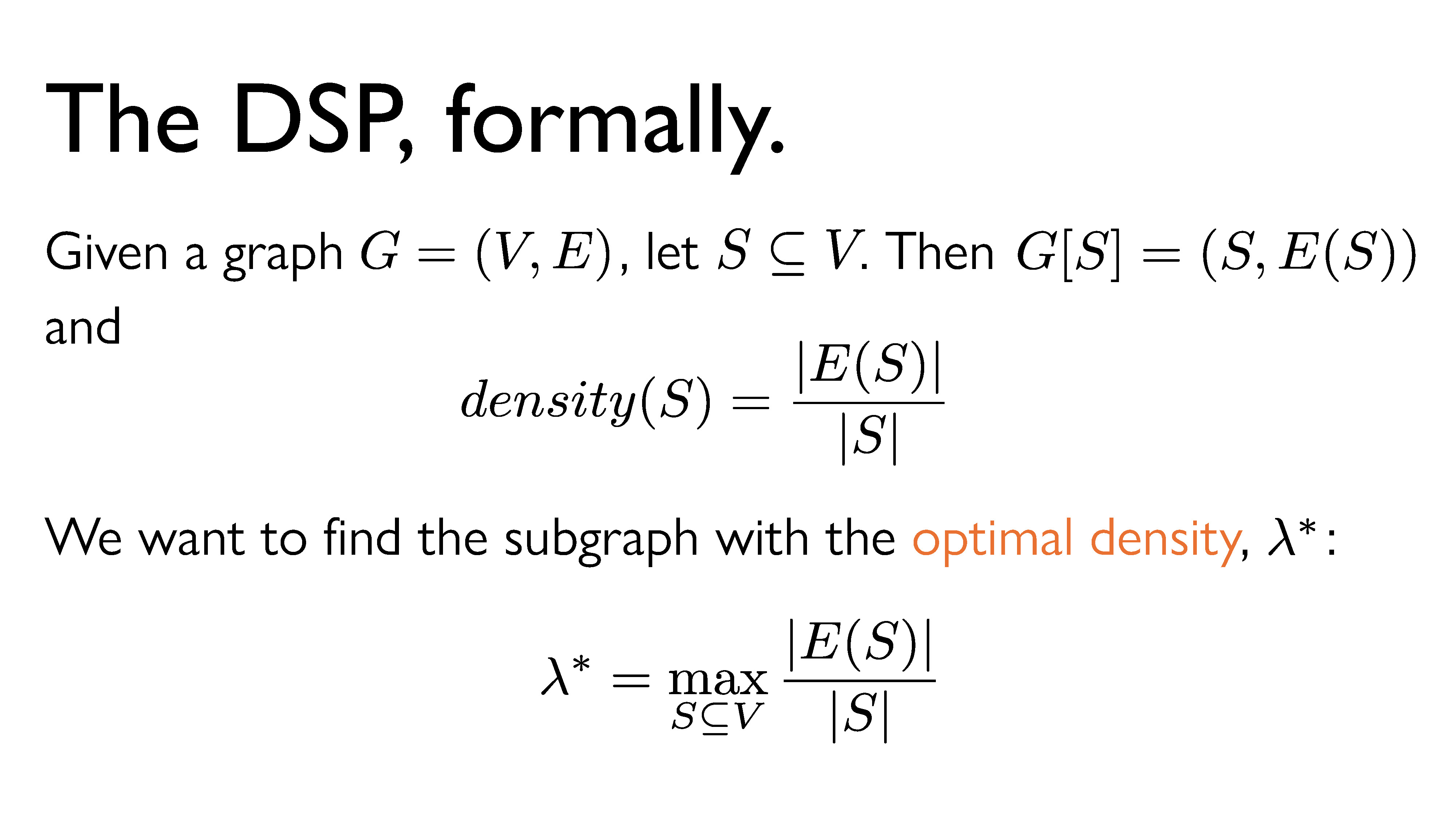
Here’s a more formal statement of the DSP: Given a graph \(G = (V, E)\) , let \(S\) be a subset of \(V\) (the vertex set of \(G\)). We define \(density(S)\) (the density of the subgraph induced by S) to be \(|E(S)|\) (the number of edges in the induced graph) divided by \(|S|\) (the number of vertices in \(S\)). We want to find the subset that maximizes the density, and we’re going to call that density the optimal density and denote it \(\lambda^*\).
Approximation Algorithms for the DSP
Now that we’re clear on what exactly the DSP is, we need algorithms that solve it for us. We have algorithms that always find the correct densest subgraph with the optimal density, but they are… not great. In theory, we can find exact solutions to this problem efficiently (that is, in polynomial time), but in practice, the algorithms that are meant to do that eat up way too much memory and never terminate.
So, we’re going to look at some sketchier algorithms today – algorithms that give us “reasonable” or “good enough” candidates for the optimal subgraph. An algorithm that gives us a reasonable answer with some sort of guarantee on the “quality” of the solution found is called an approximation algorithm (I’ve written more on those here), and we’ll mainly be looking at two of them here.
Peeling
The first algorithm we’re going to look at is called peeling1, which dates back to around the year 2000 and is actually used in the real world. The idea is that we peel away vertices of low degree: this means that at each peeling step, we remove the vertex with the lowest degree, as well as all of the edges that are attached to it. As we continue to peel vertices, the density of the graph changes – at some points it may increase, and at other points it may decrease. We keep track of the density of the graph at every point, and the point in our peeling at which the density was highest is our “candidate” for the densest subgraph.
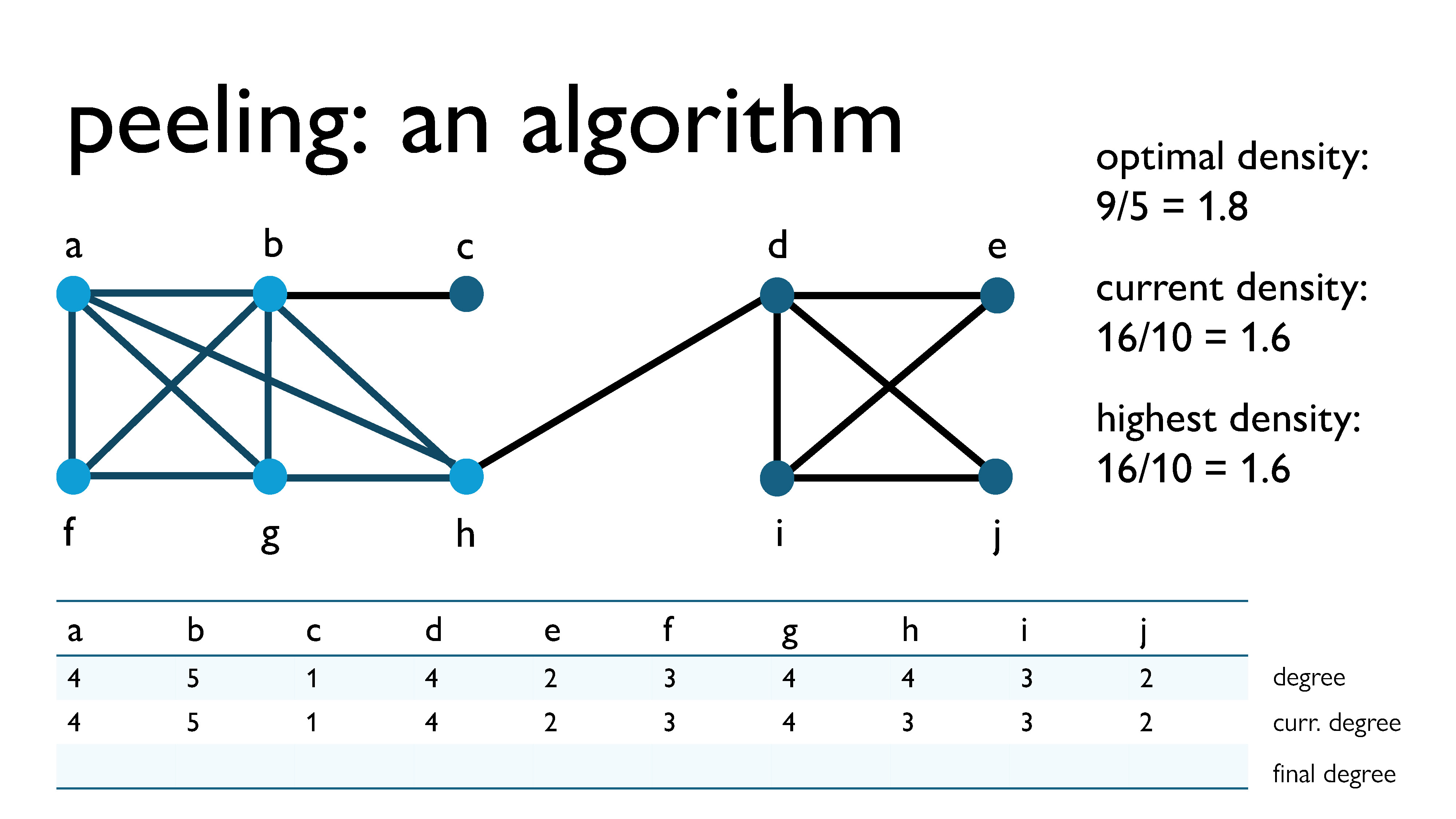
Here’s an example graph I’m going to use to demonstrate the peeling process. The part of the subgraph that is highlighted in blue is the actual densest subgraph, which I manually computed in advance. I’ve also put a table at the bottom of the slide, where you can see what the degrees of the vertices are as we peel them away, as well as some information about the density of the graph on the side. I’m going to peel away the vertices, and then we’re going to see which candidate the algorithm gives us for the densest subgraph.
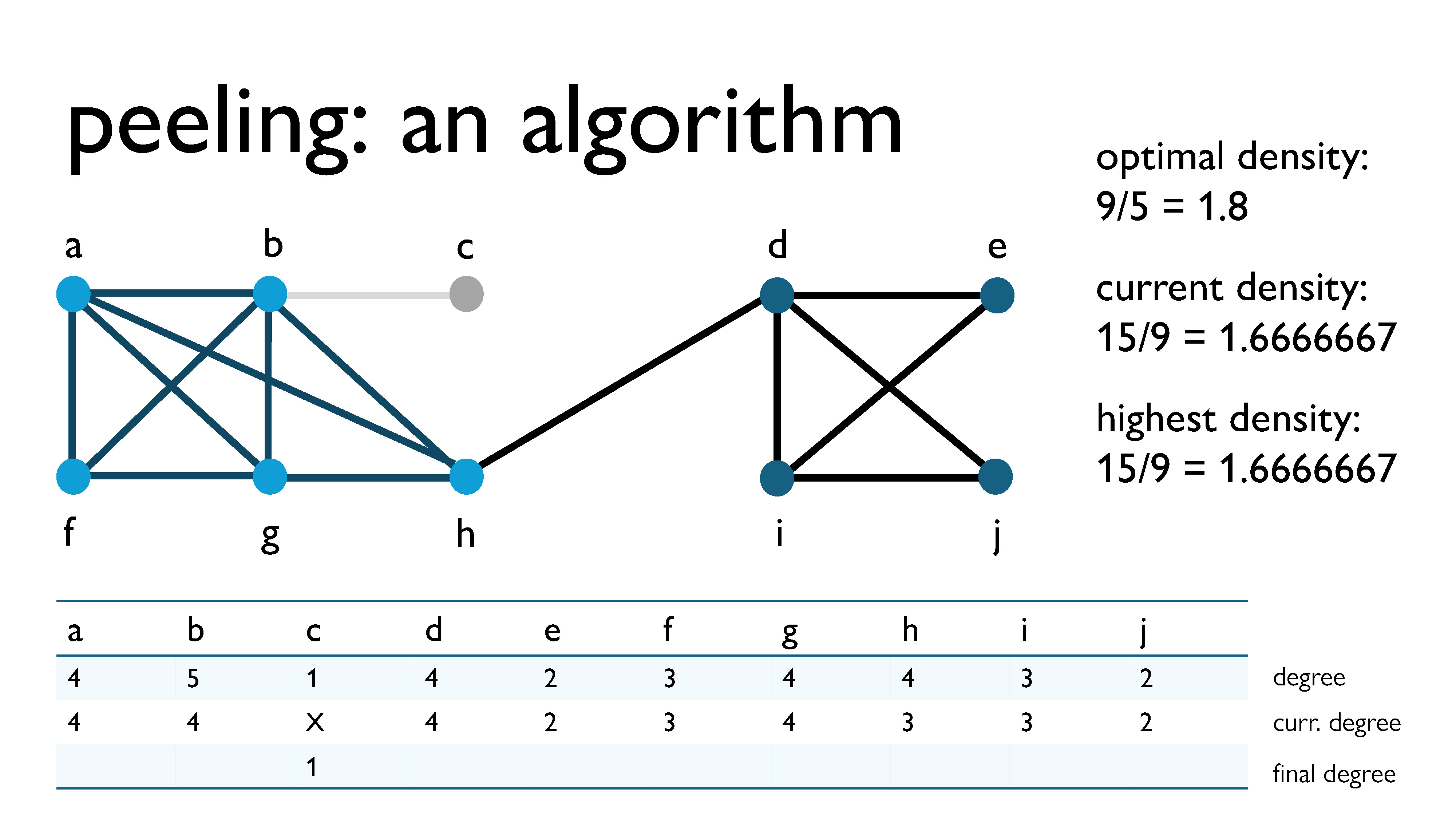
First, we peel vertex \(c\), because it has the lowest current degree (\(\text{curr\_deg}(c) = 1\)). This now becomes its final degree.
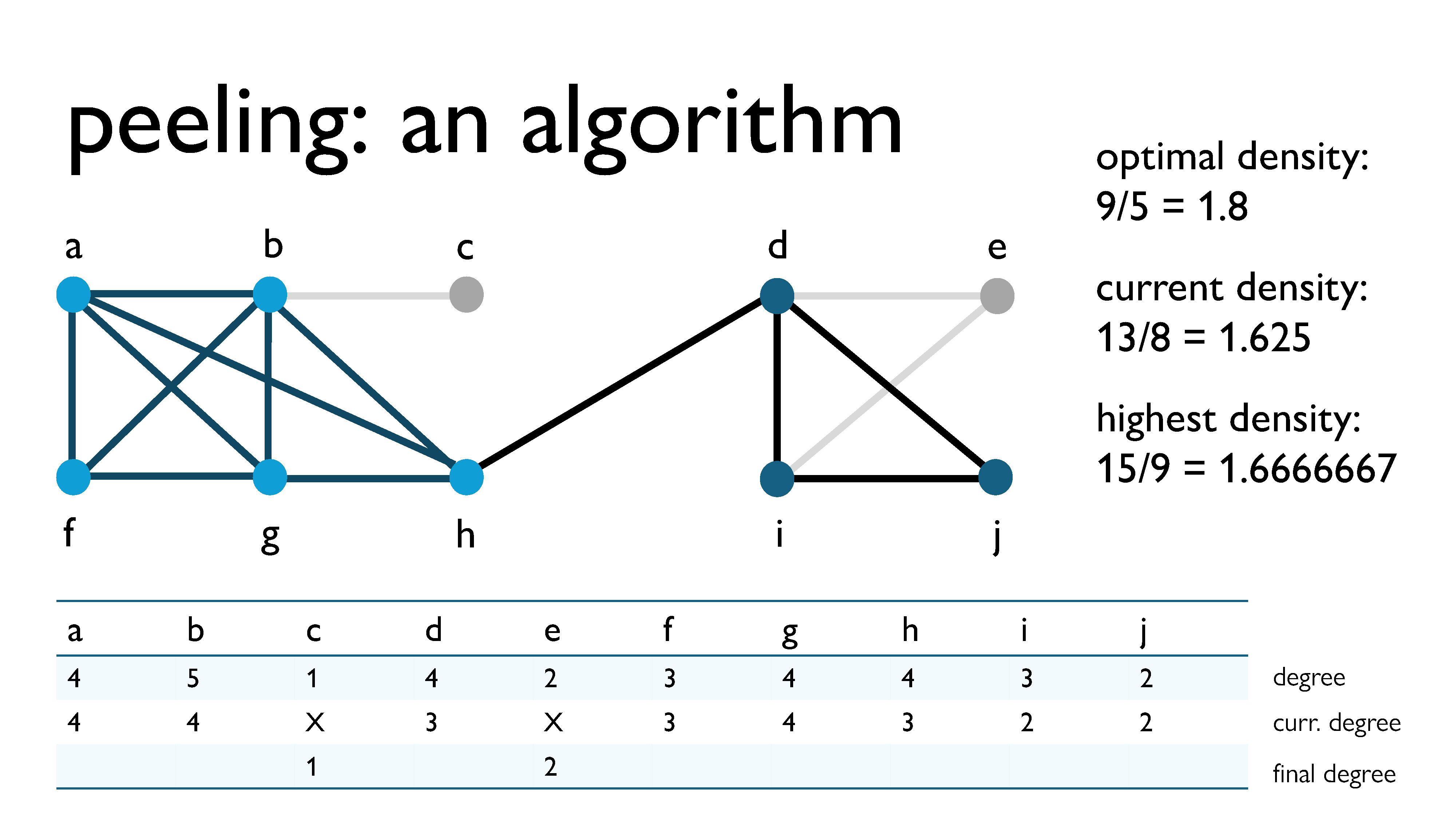
Then, we peel vertex \(e\), because it has the lowest current degree (\(\text{curr\_deg}(e) = 2\)). This now becomes its final degree.
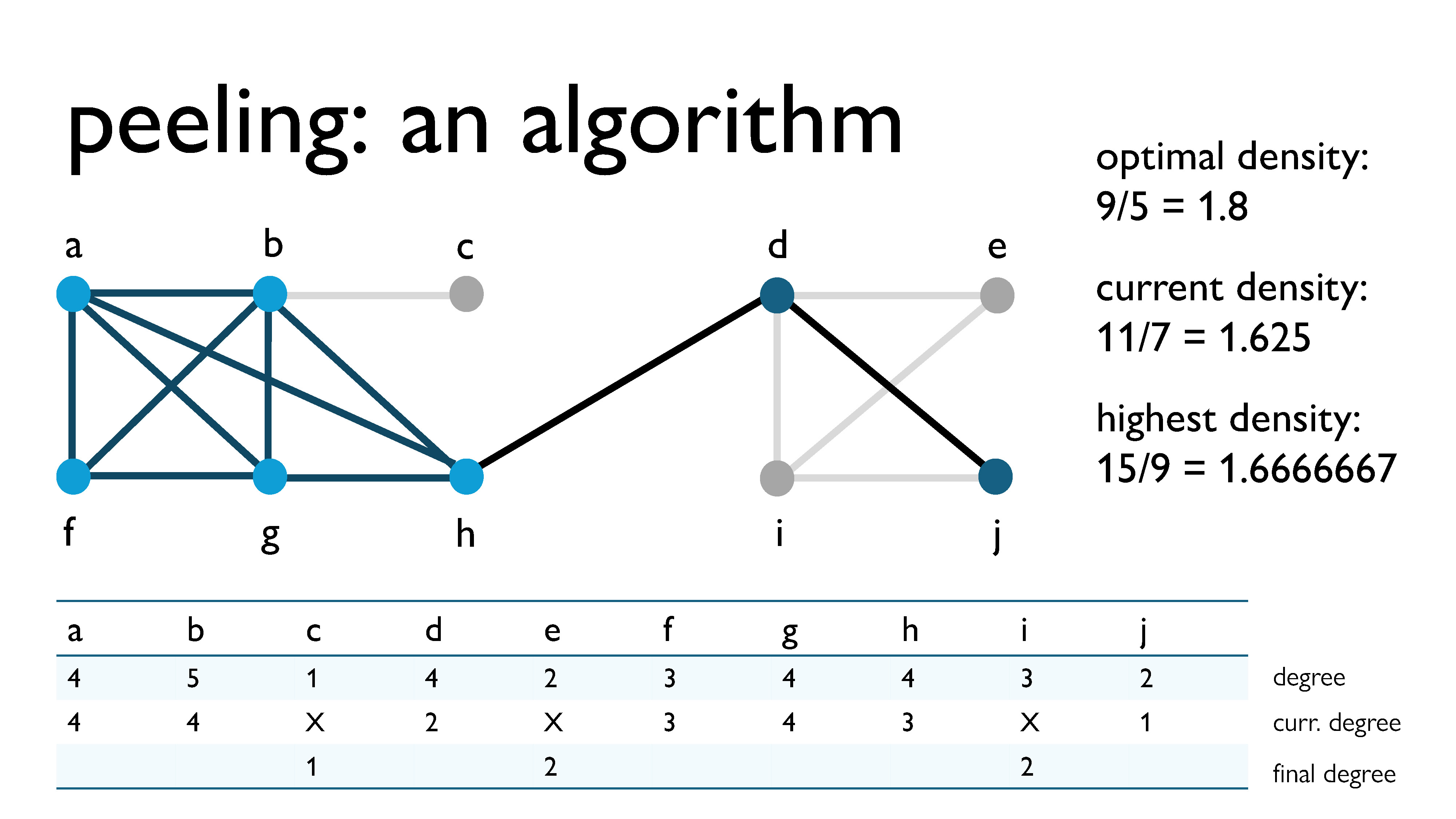
We repeat this process with all of the other vertices. Here, we’re peeling vertex \(i\), with a current degree of 2.
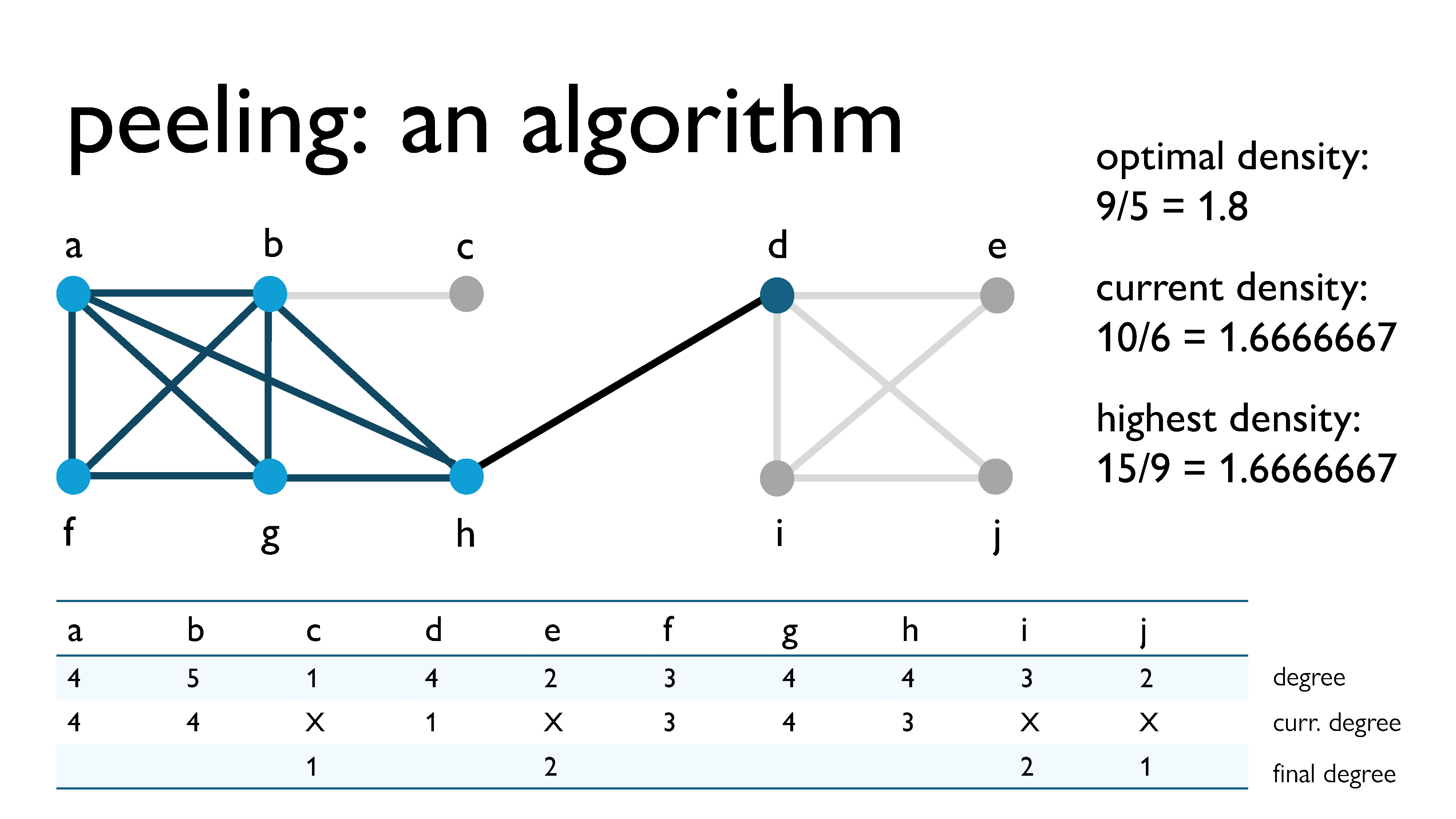
Here, we’re peeling vertex \(j\), with a current degree of 1.
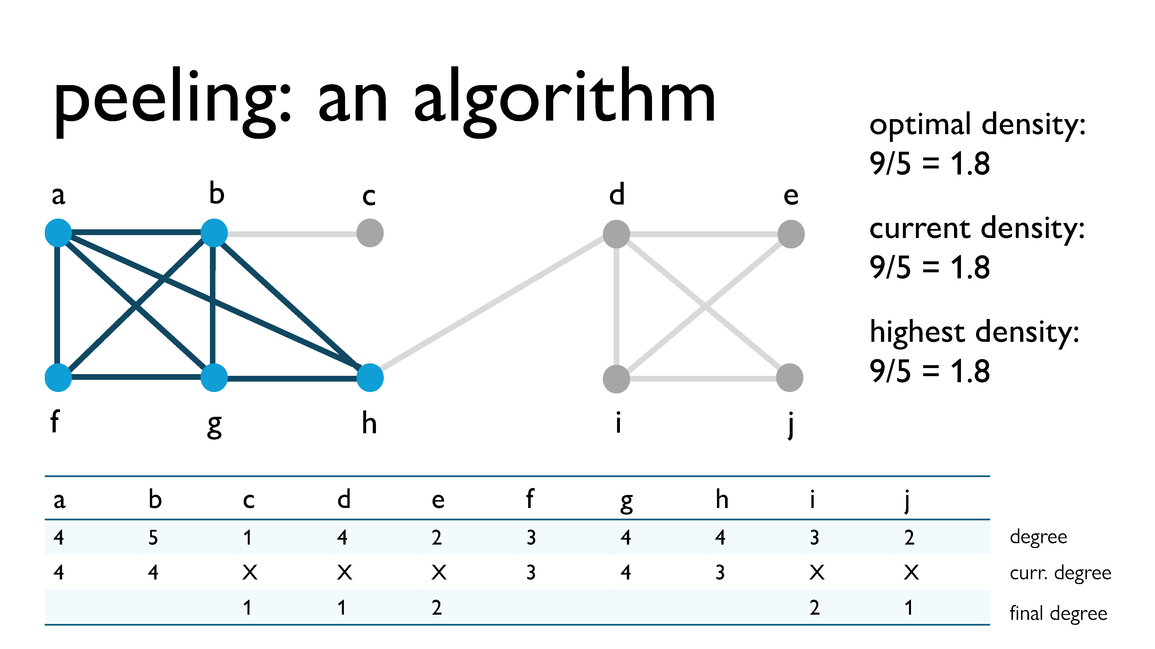
Here, we’re peeling vertex \(d\), with a current degree of 1.
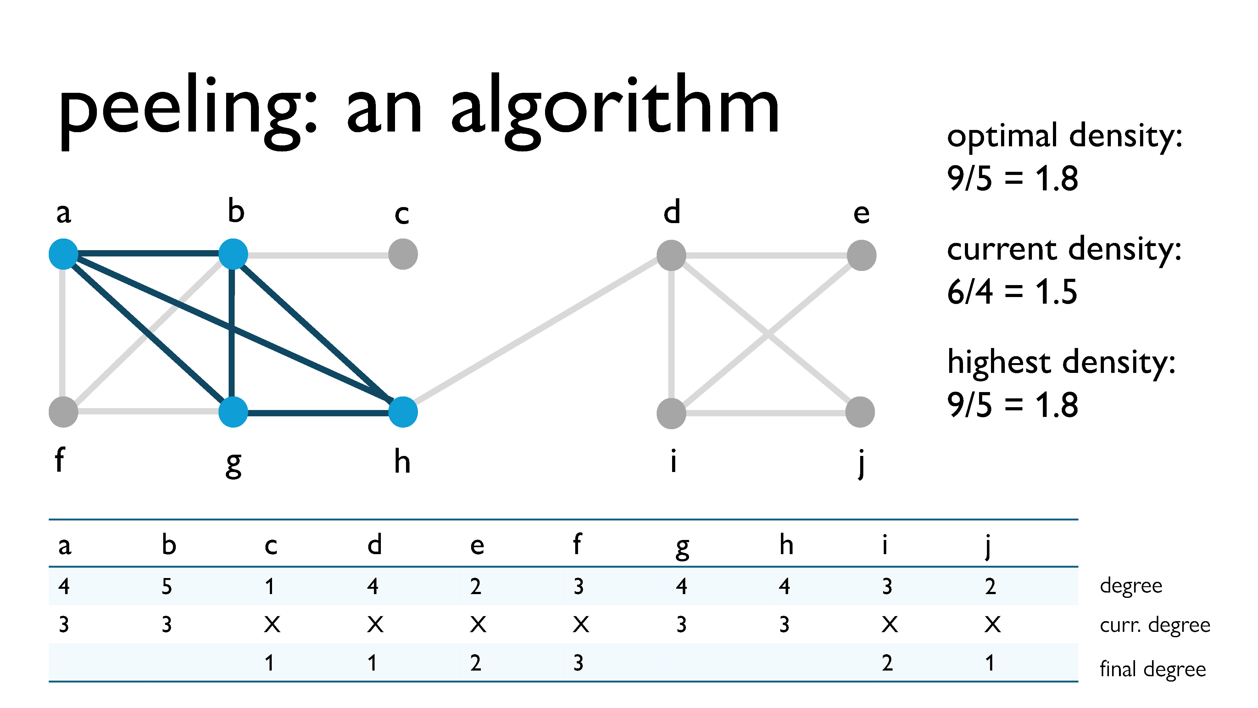
Here, we’re peeling vertex \(f\), with a current degree of 3.
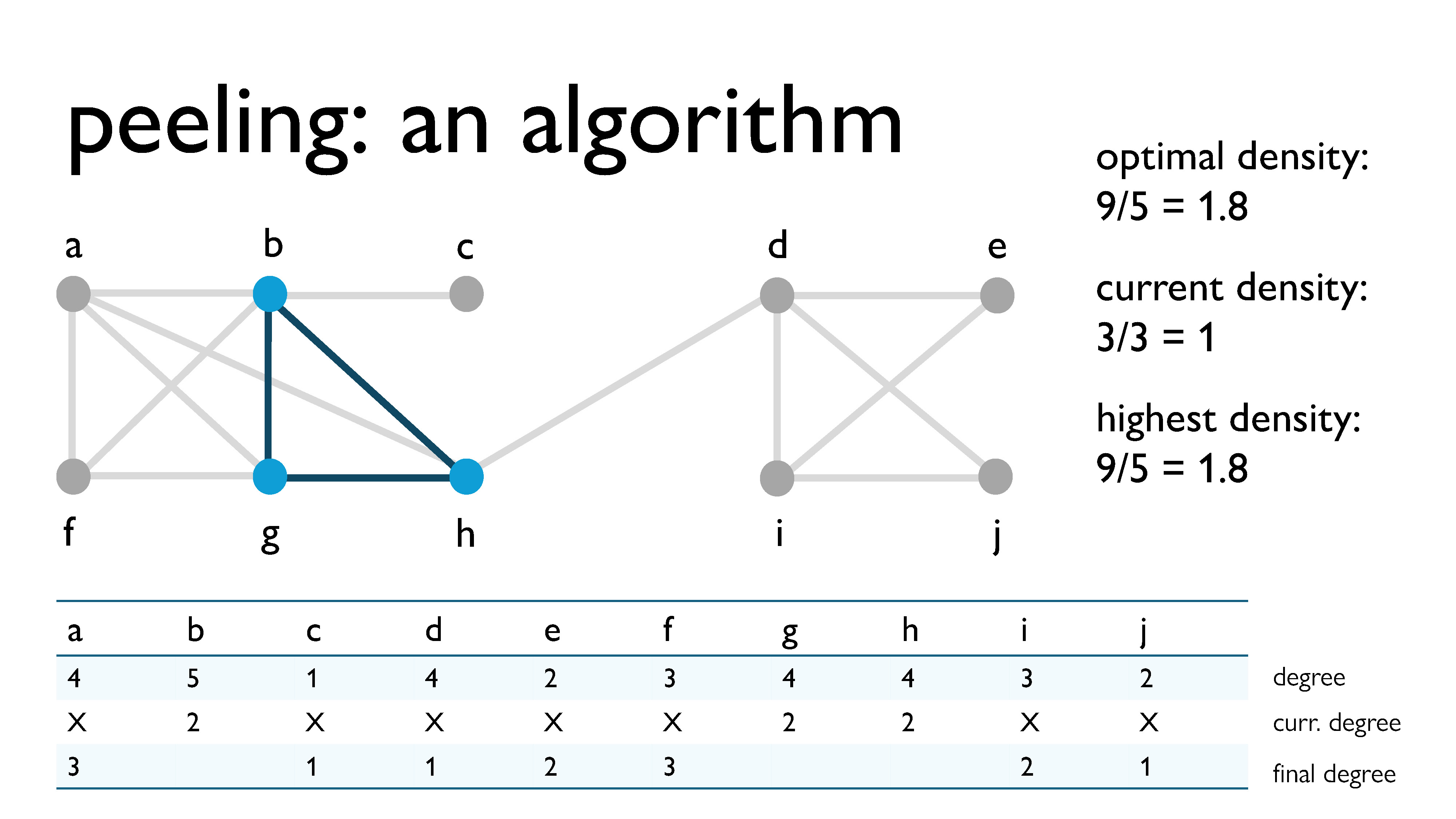
Here, we’re peeling vertex \(a\), with a current degree of 3.
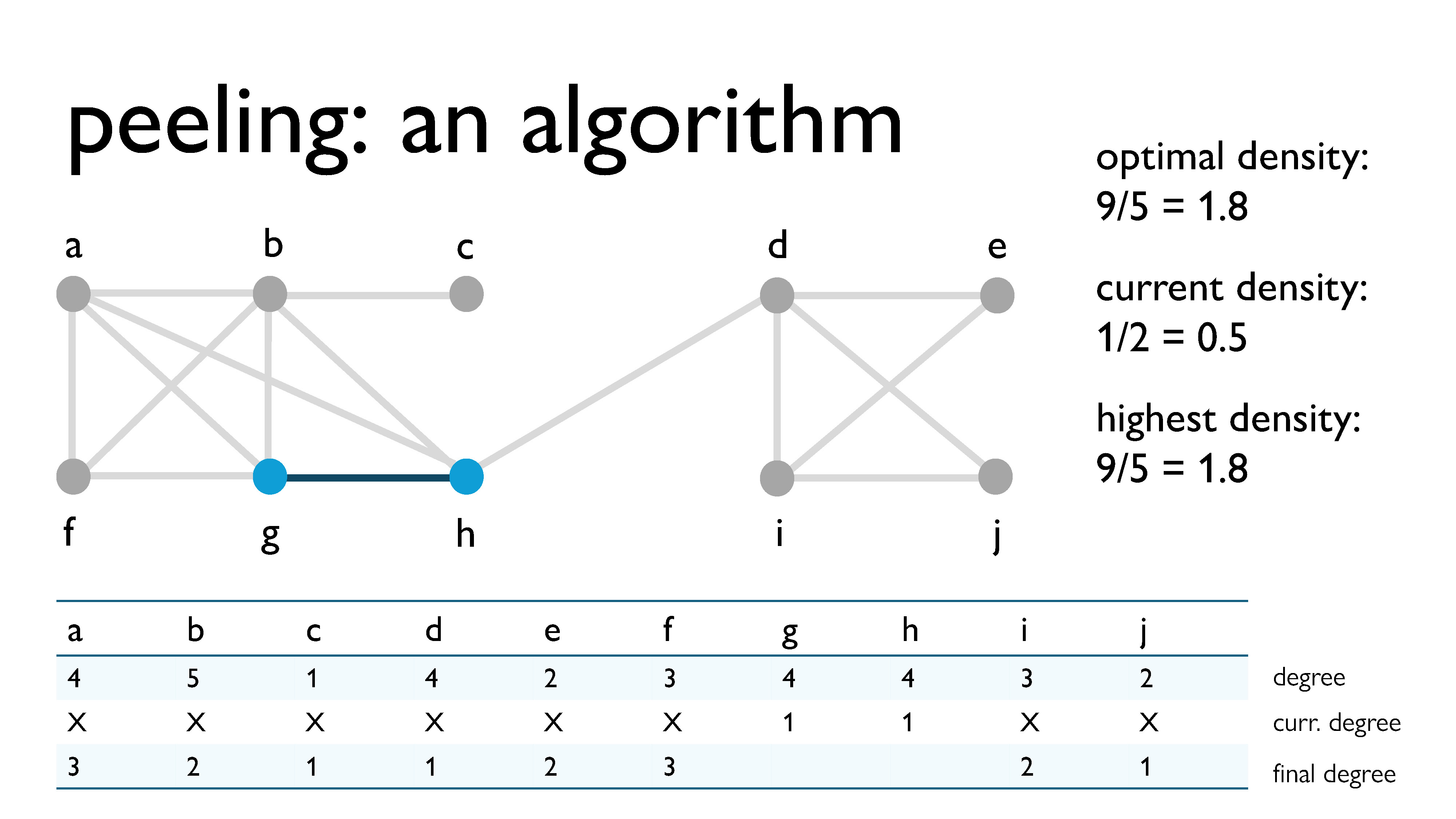
Here, we’re peeling vertex \(b\), with a current degree of 2.
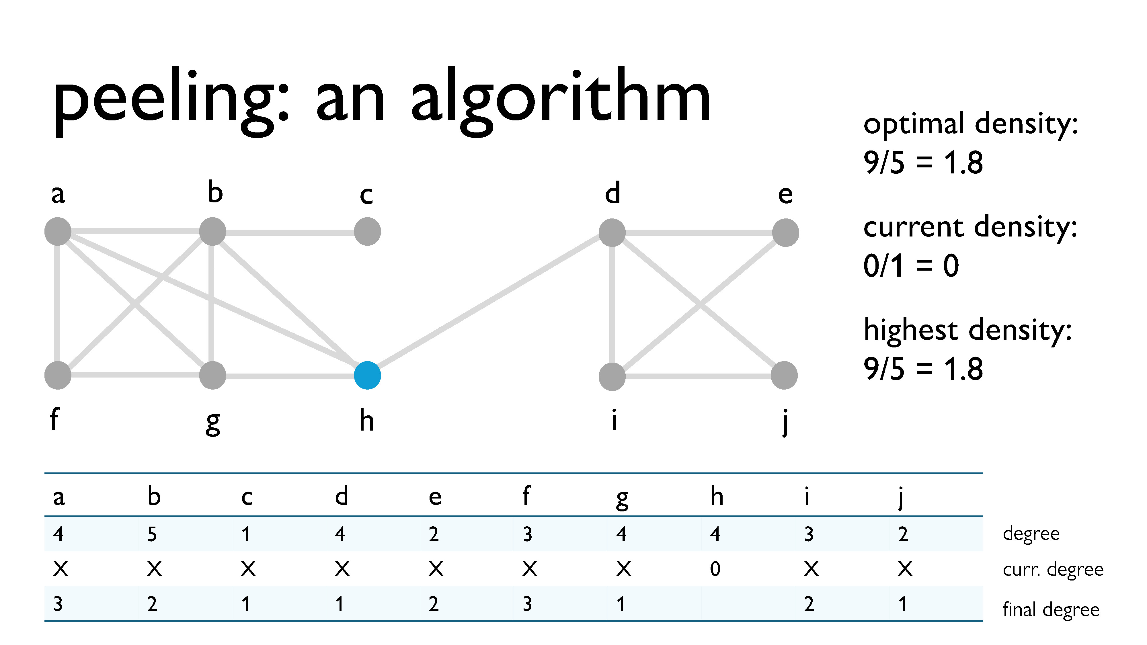
Here, we’re peeling vertex \(g\), with a current degree of 1.
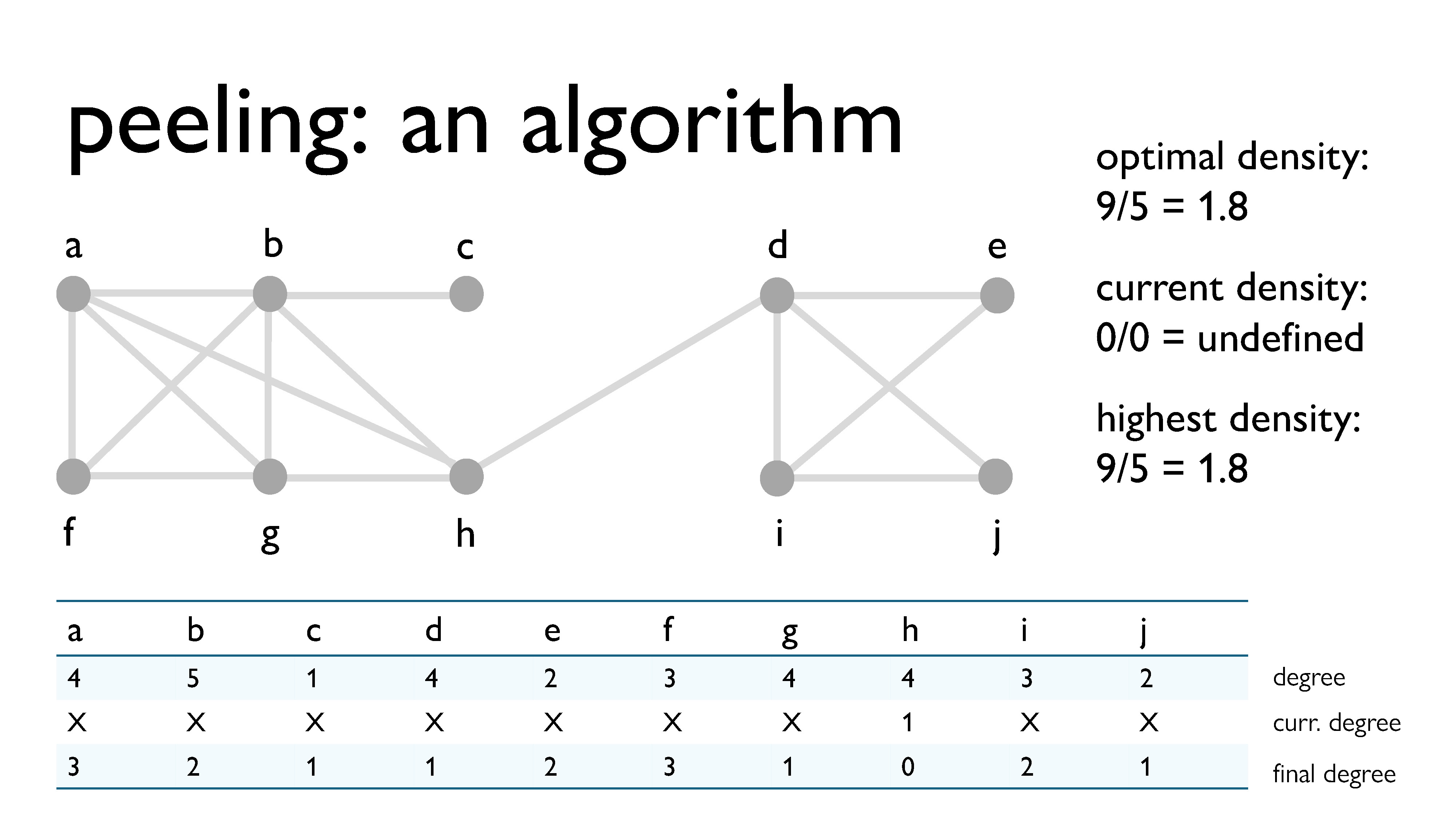
Finally, we peel vertex \(h\), with a current degree of 0.
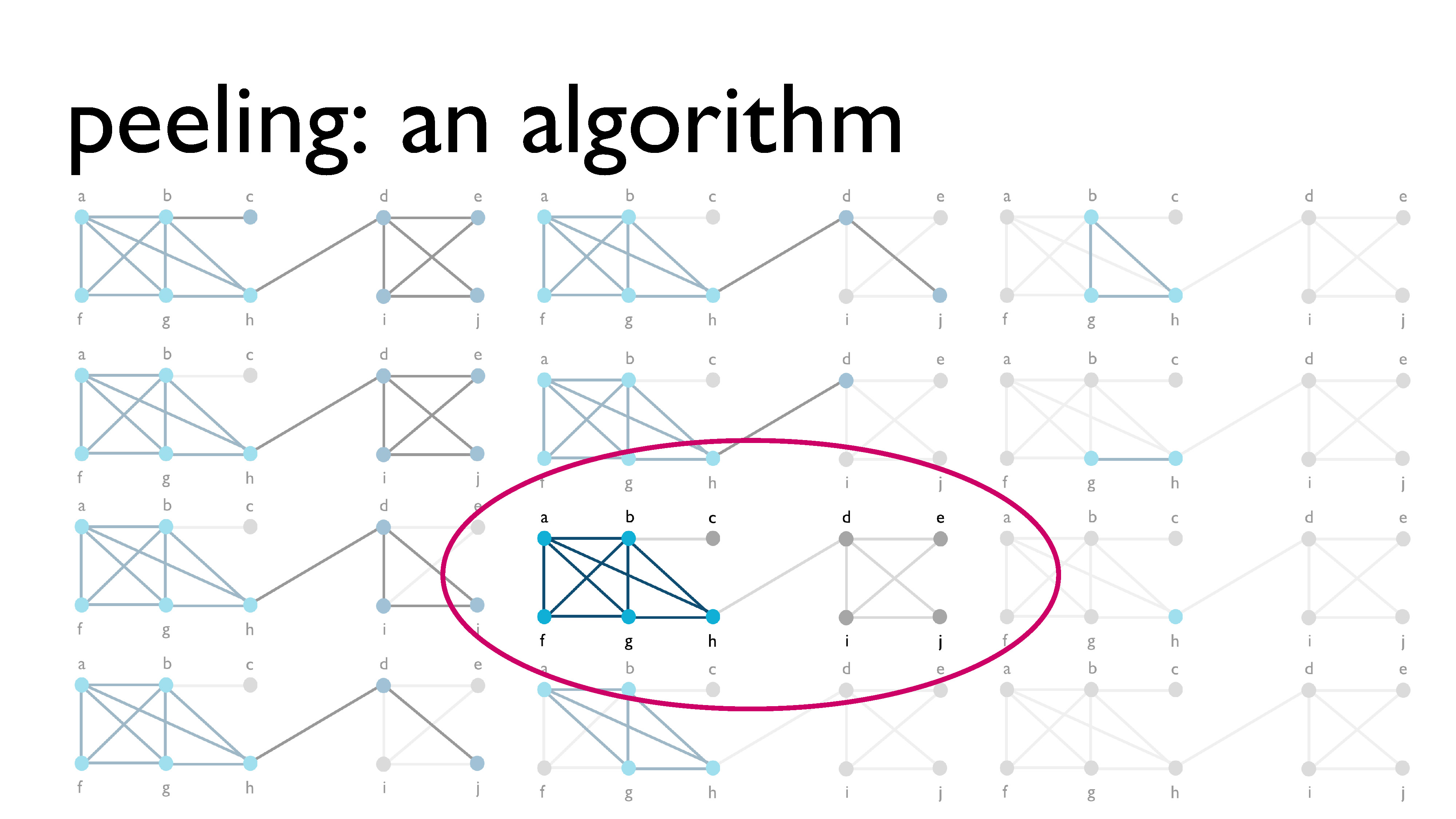
Now that we’ve peeled all of the vertices, we look back at all of the different subgraphs we had over the course of the process, and we choose the subgraph with the highest density, which is what you see circled here in pink.
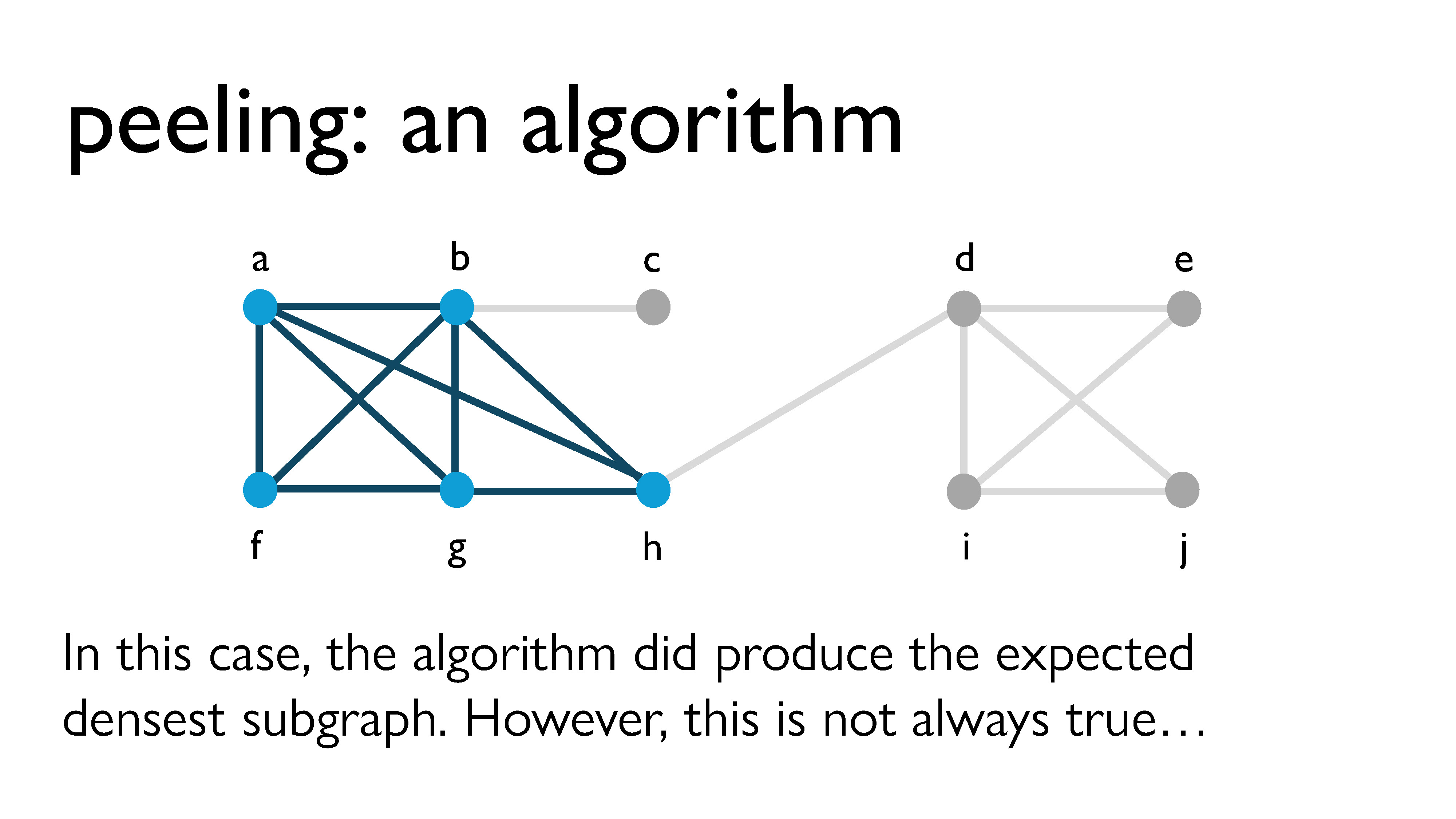
In this case, peeling did produce the correct densest subgraph. But it doesn’t always work exactly. In fact, peeling usually doesn’t quite work.
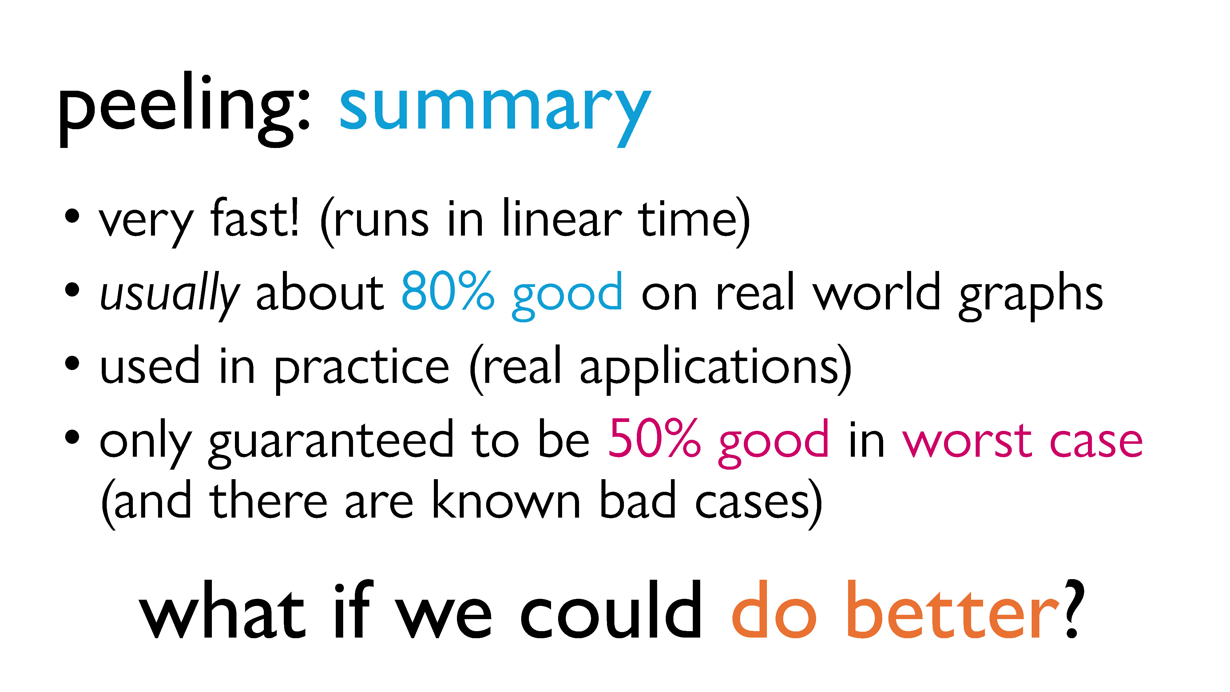
If we summarize our results from peeling, it is very fast! It runs in linear time. Usually, the graph it produces is about 80% as good as the actual densest subgraph. For a linear time algorithm, this is great, which is why it’s actually used in practice. However, it’s only guaranteed to be around 50%, and there are known “bad graphs” where that bound is tight. So what if 50% isn’t good enough for me? Can we do any better? This is where the idea of iterative peeling comes in.
Iterative Peeling
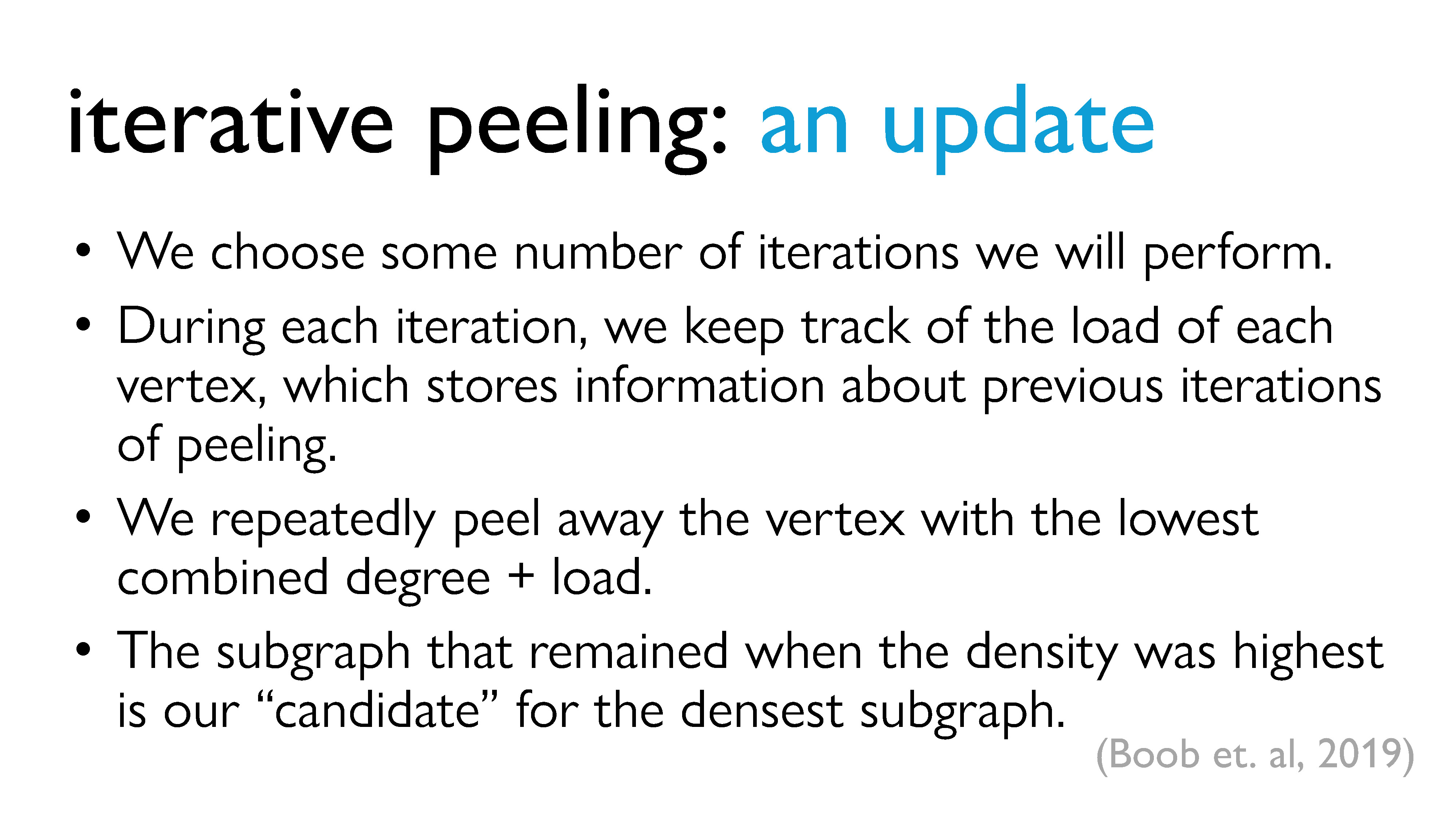
In around 2019, some researchers proposed that one way to improve the accuracy of our approximation could be to just repeat this peeling procedure over and over. The idea is that we first decide on the number of peeling iterations we are going to perform, where one iteration is a full cycle of peeling. During each iteration, in additional to keeping track of the current degree of each vertex, we keep track of a new piece of information called the load, which more or less stores information about the previous iterations. Instead of peeling based on the degrees of the vertices, we repeatedly peel away the vertex with the lowest combined current degree + load. Again, at each point, we keep track of the remaining subgraph, and the subgraph with the highest density becomes our candidate for the densest subgraph.
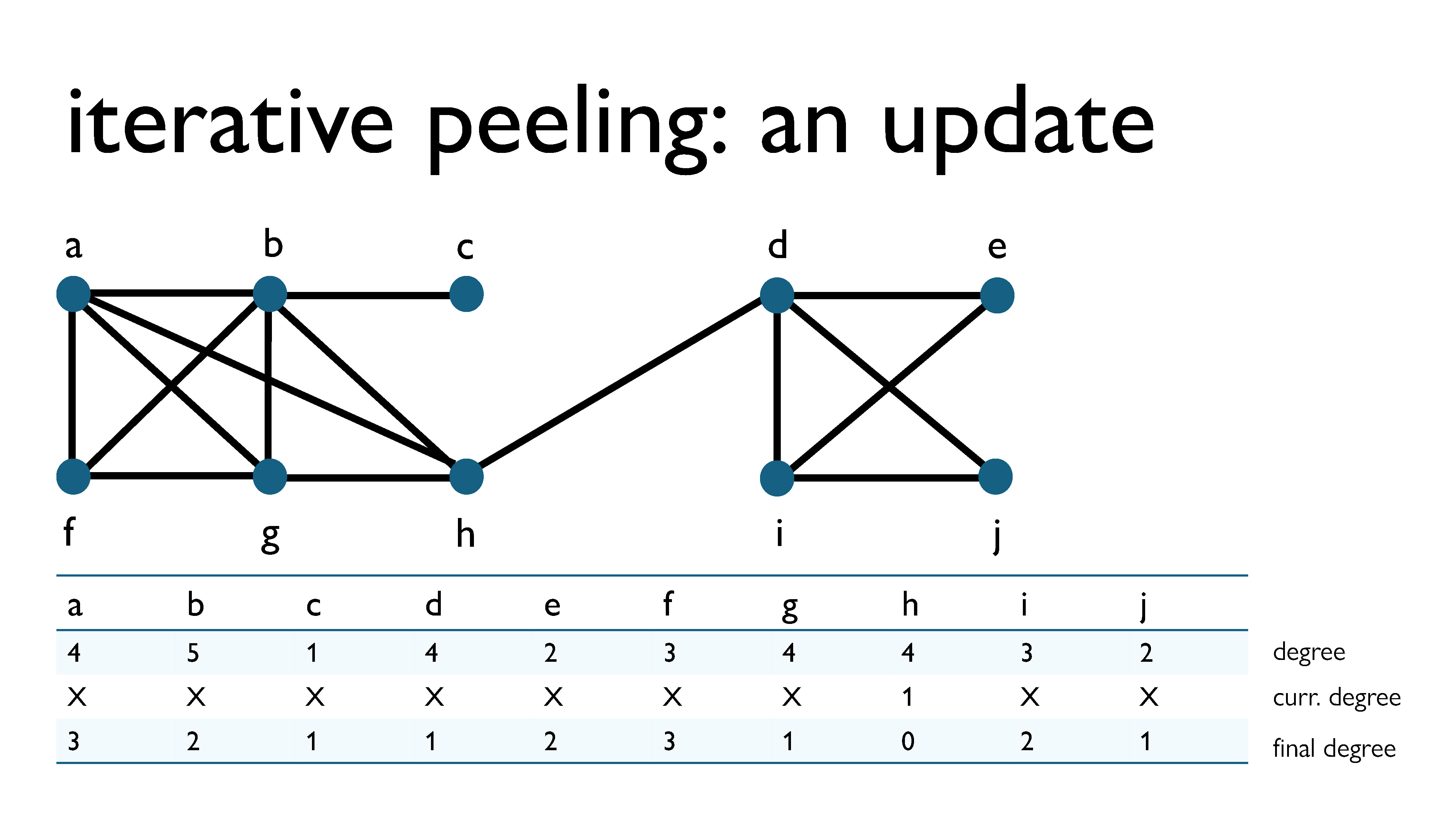
So how does this work? The first iteration of iterative peeling is exactly the same as a cycle of regular peeling, since we initialize the loads of all of the vertices to zero. So, let’s pick up from where we left off in the earlier peeling example. As you can see in the image above, in the previous example, we kept track of the degree of every vertex at the time when it was removed. You may have noticed me keeping track of this, and not known why. However, the degree at the time of removal gets added to the load of the vertex at the end of every iteration.
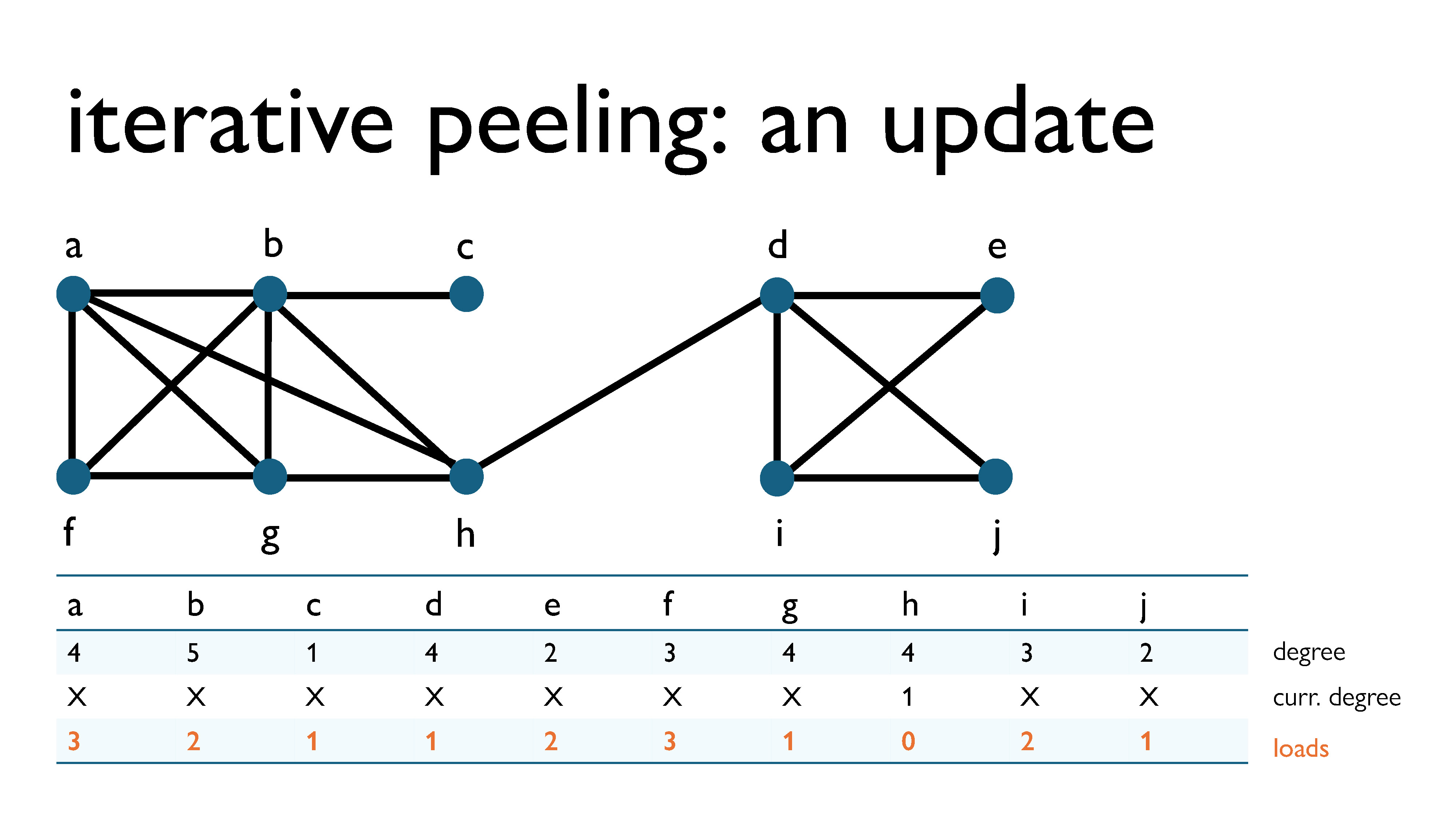
Since the load before the first iteration was 0 for each vertex, the load of each vertex after the first iteration will be equal to its degree at the time of removal.
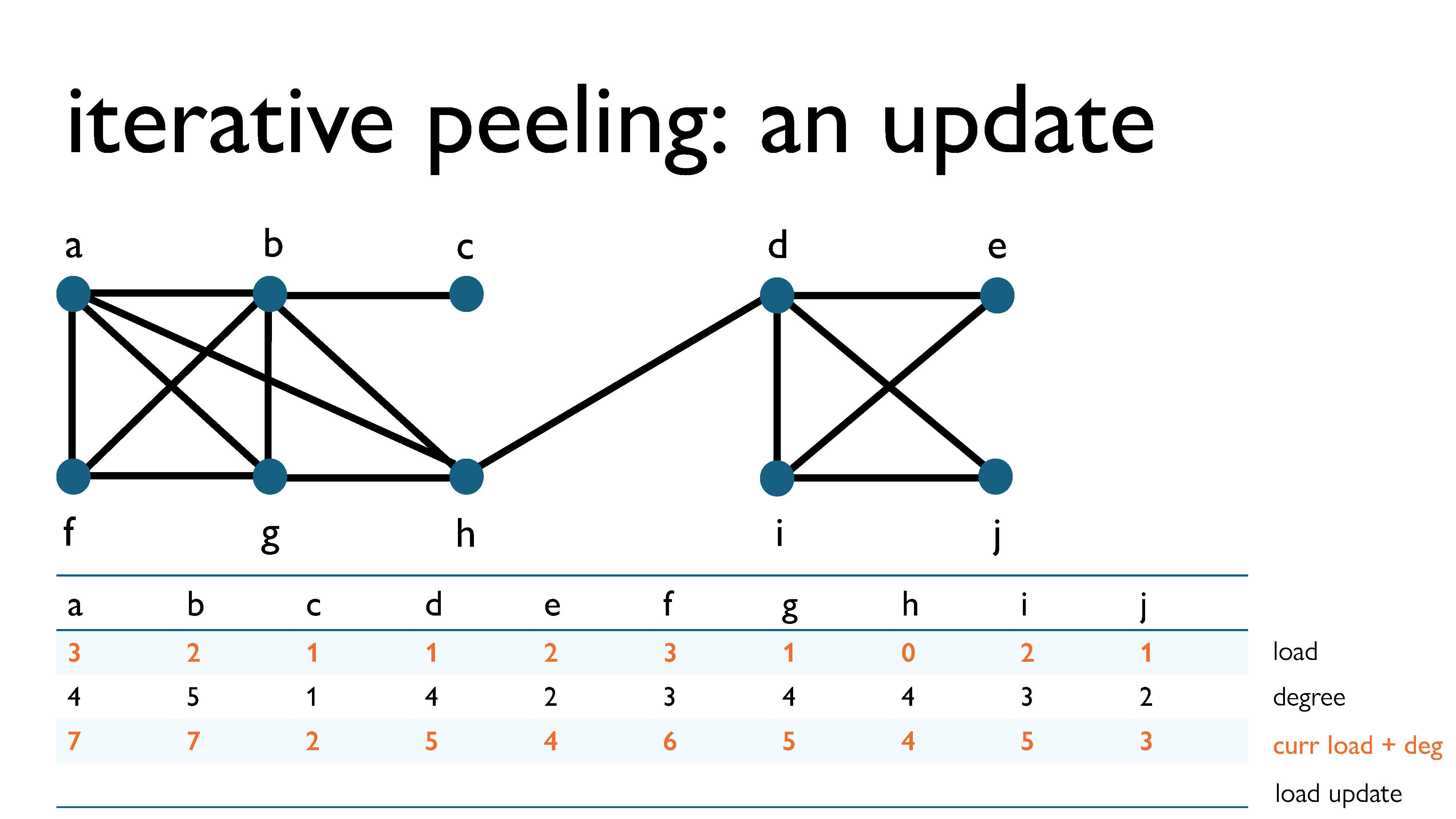
We can now update this diagram to keep track of loads, degrees, the current load + deg, and the load update (the value that will be added to the load after this iteration).
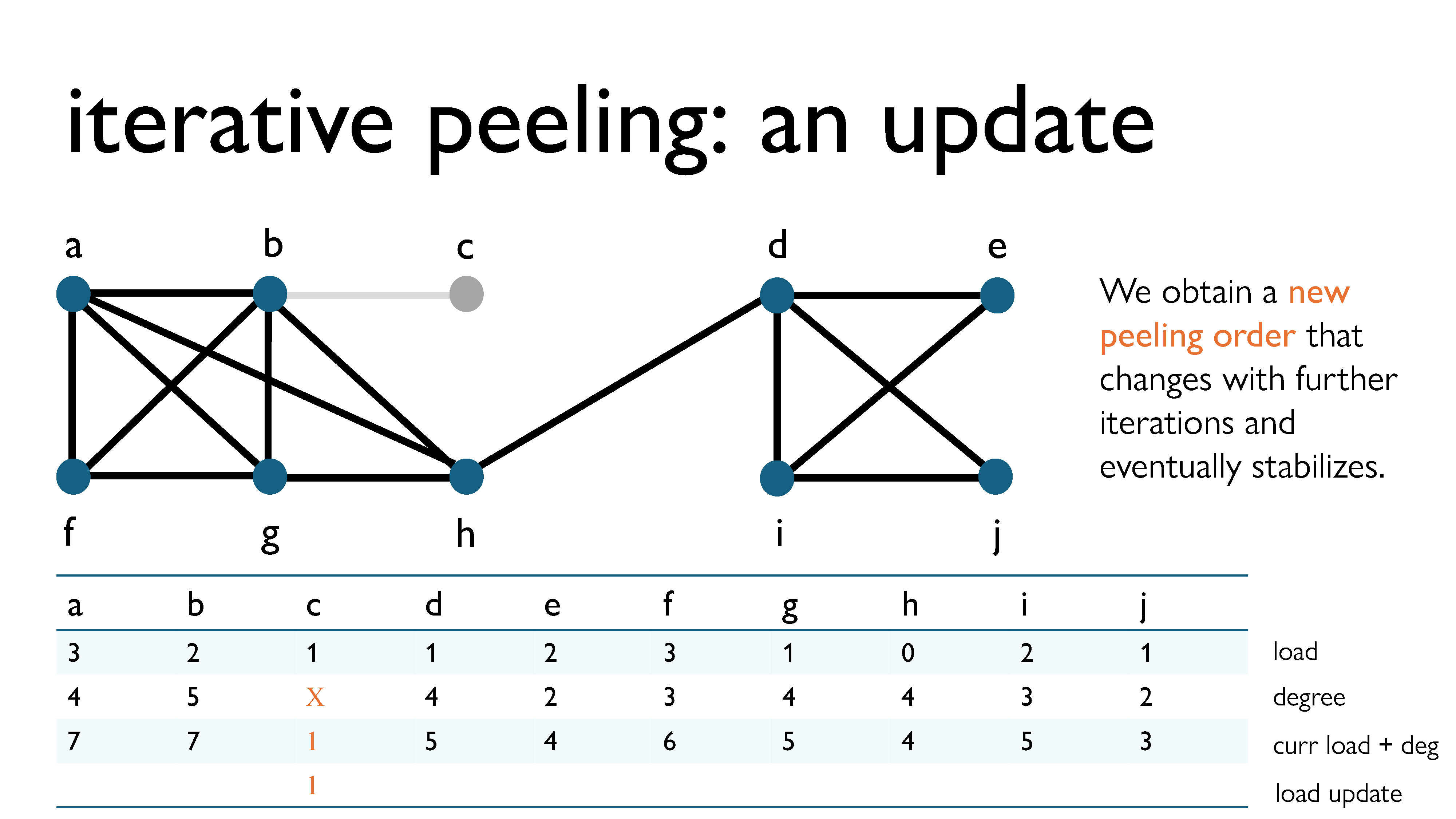
Here’s the first peeling step. We removed vertex c, since it had the lowest load + current degree in the graph. Since it had degree 1 at the time of removal, in the next iteration it will have load 1 (its current load) + 2 (its degree when removed) = 2.
What’s interesting is that with this new technique, the peeling order will begin to evolve with each iteration, and eventually, with enough iterations, it should stabilize itself.
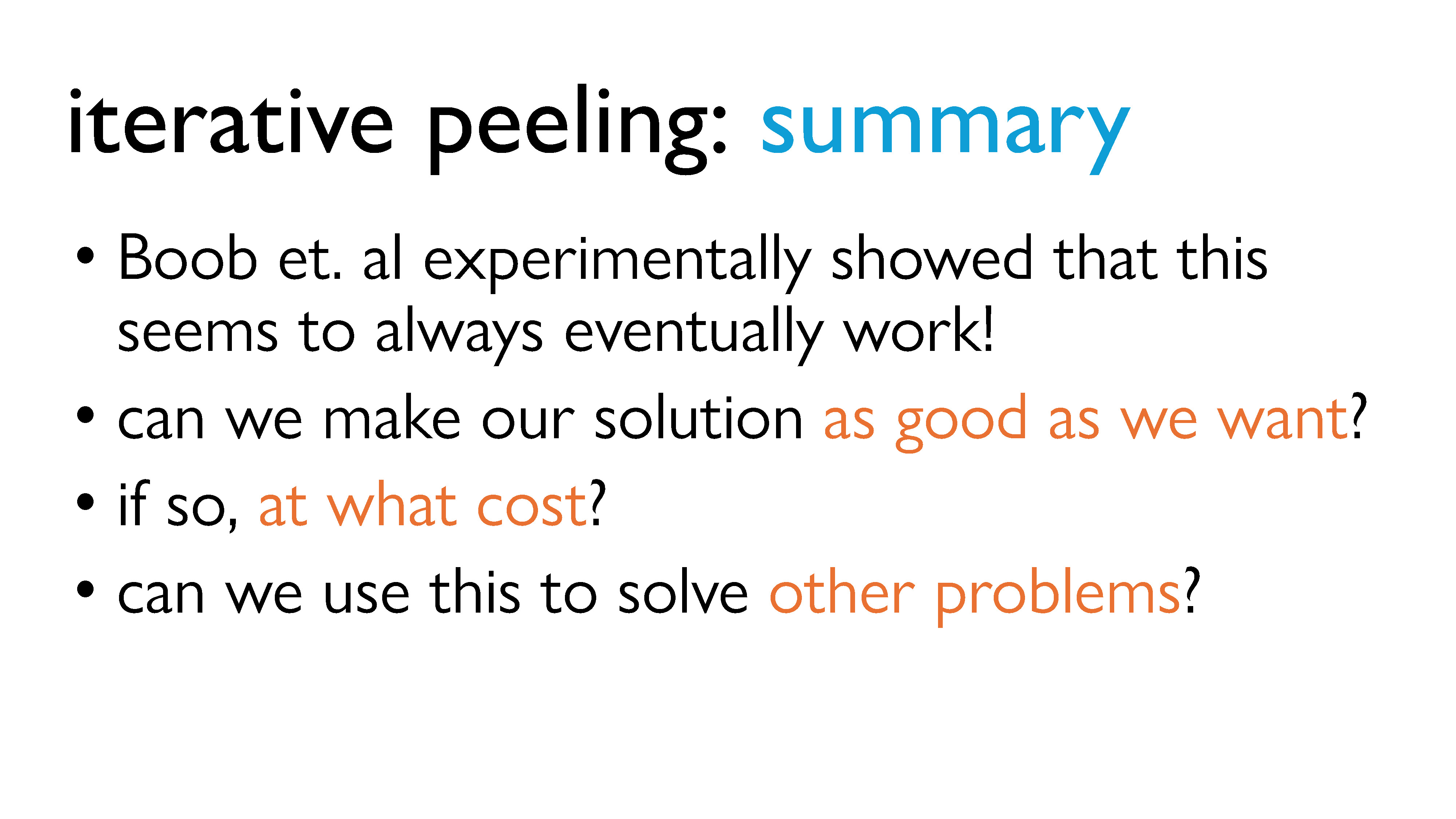
As you’ve probably noticed, it seems like if we do this procedure enough times, we’re always eventually going to get the optimal subgraph. But we don’t know if this is actually true, right? We hope it is, but we don’t really have a way to prove this right now. Also, this is a really simple procedure; like, it’s relatively simple to implement (which I actually spent a summer doing) and I could probably explain it to a ten-year old. So it would be really nice if we could use this method to solve other problems.
So it turns out that we can actually can answer these questions. We’re going to generalize a little bit, and do a bit more abstraction, but it is doable. We’ll look more into that in Part 4.
Part 4: Set Functions, Supermodularity and the Densest Supermodular Set Problem
Digression: Submodularity, Modularity, Supermodularity, and Set functions
In Part 3, we discussed the densest subgraph problem (DSP) and some algorithms for solving it. In this section, we’ll be looking at how we can generalize this problem and those algorithms to solve some other problems.
We’re going to go on a detour for a while now. This is the scary section. It was scary for me, and it’ll probably be scary for you too, but we’ve gotten this far together. This is the part of the talk where I will introduce some fancy new math I had to learn in order to understand how one might generalize iterative peeling to solve adjacent problems.
As a preview of where I’m going with this, it turns out that iterative peeling works because the densest subgraph problem is a special case of something called the “densest supermodular set problem”. (Don’t worry, I’m going to break down what that means; that’s what this whole section of the talk is about.) Rephrasing the DSP in terms of this “supermodularity theory” gives us a unifying framework that explains the differing “error rates” between peeling and iterative peeling and also gives us a way to maybe get solutions to some related problems for free. We’re going to be getting a glimpse of how theoretical concepts are used to extend existing solutions to problems to other contexts.
So we’re going to learn some new ideas here, and we’re going to make some older ones precise. I think for some of you, “examples” might be the only word you recognize, whereas for others, some of this may be vaguely familiar. Either way, that’s okay. This is your moment to freak out.
*deep breath*
Alright, time’s up. Let’s get started.
Set Functions
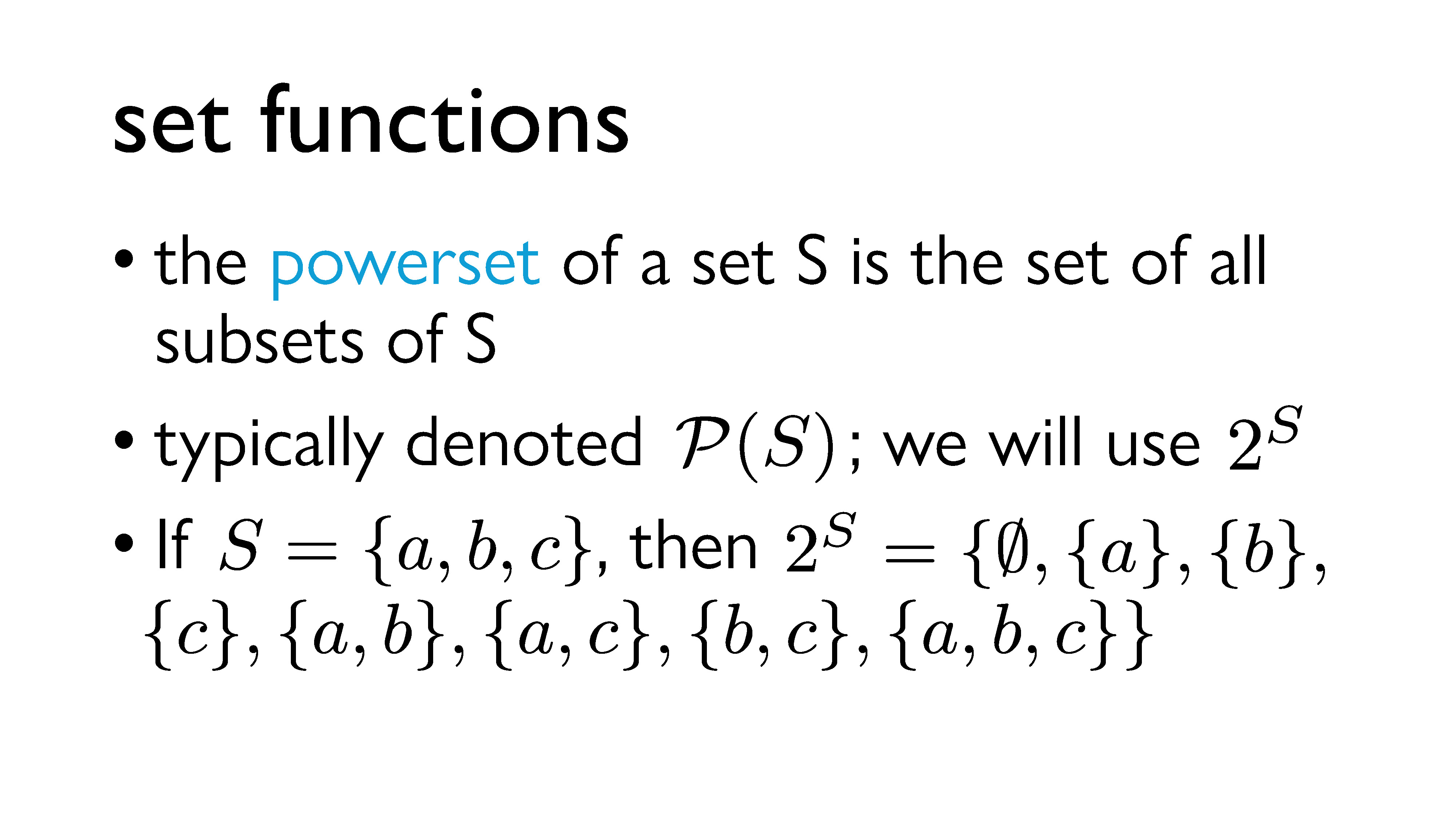
We’re going to kick off by talking about sets and set functions. As you likely remember from high school, a set \(S\) is an unordered collection of distinct objects. The powerset of \(S\) is the set of all subsets of \(S\), which includes both the empty set (denoted \(\\{\\}\) or \(\emptyset\)) and \(S\) itself. Typically, this is denoted \(\mathcal{P}(S)\), but we’re going to use this alternate \(2^S\) notation2, which is equivalent.
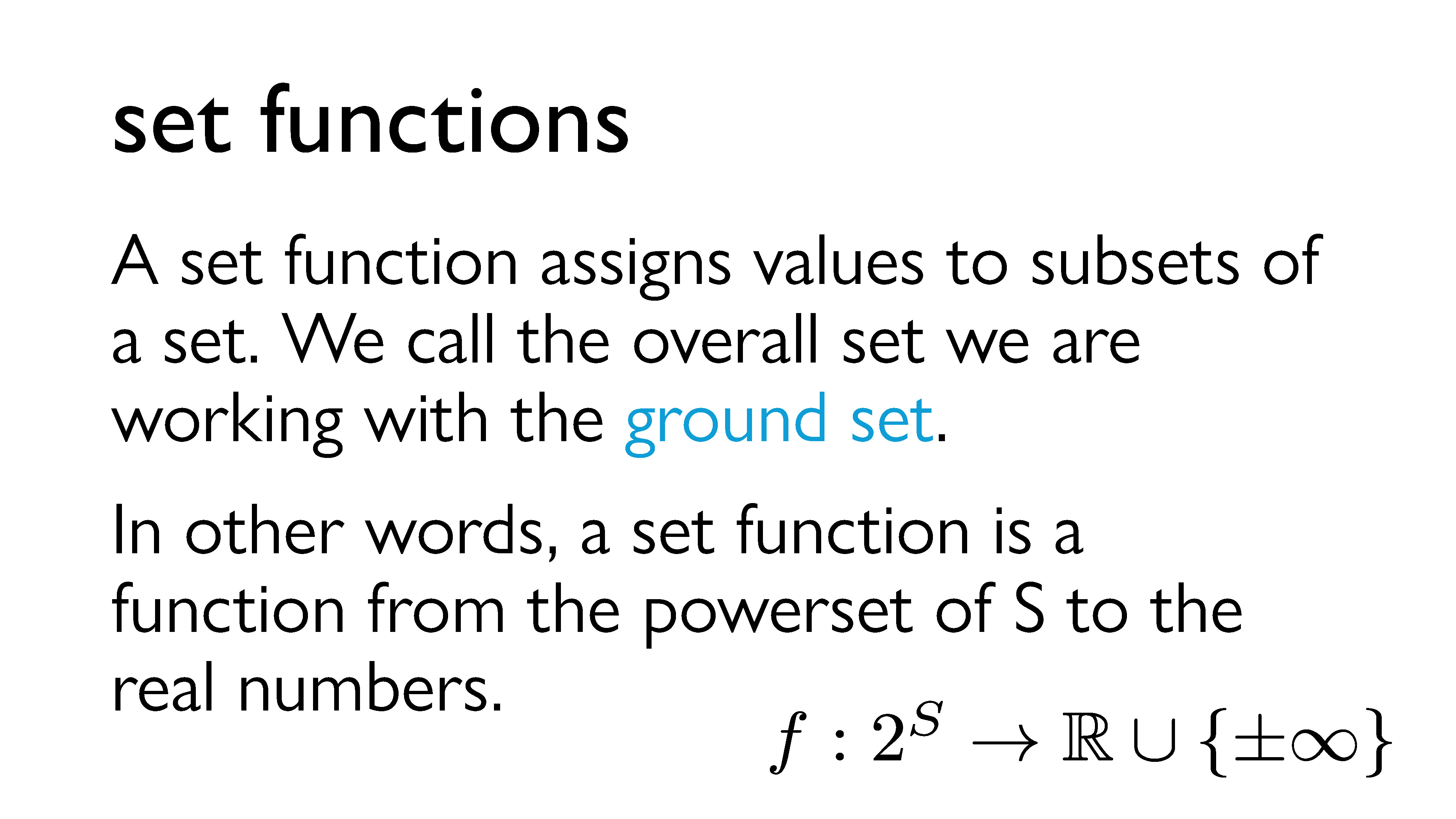
A set function \(f: 2^S \rightarrow \mathbb{R}\cup \{\pm\infty\}\) is a special type of function that assigns a value to each subset of a set. First, a specific set we will be working with is defined, and we call that set the ground set. (This is \(S\).) Then, we map every subset of the set to a real number (sometimes including positive and negative infinity). For example, if \(S = \\{a,b\\}\), we might map \(\emptyset\) to 0, \(\\{a\\}\) to 1, \(\\{b\\}\) to -2.5, and \(\\{a, b\\}\) to 0.
In short, a set function is a function from the powerset of the ground set to the real numbers.
From this point on, we’re going to be using \(S\) to mean some arbitrary subset, so we’re going to call our ground set \(V\) instead. Here’s some useful terminology for different types of set functions.
Let \(f : 2^V \rightarrow \mathbb{R}\). \(f\) is called: - normalized if \(f(\emptyset) = 0\) - monotone increasing if \(A \subset B \implies f(A) < f(B)\) - monotone decreasing if \(A \subset B \implies f(A) > f(B)\) - additive if \(f(A \\,\dot\cup\\, B) = f(A) + f(B)\) (that is, if for any disjoint sets \(A\) and \(B\), the union of \(A\) and \(B\) has a value equal to the sum of the values of \(A\) and \(B\)) - subadditive if \(f(A \\,\dot\cup\\, B) \leq f(A) + f(B)\) - superadditive if \(f(A \\,\dot\cup\\, B) \geq f(A) + f(B)\)
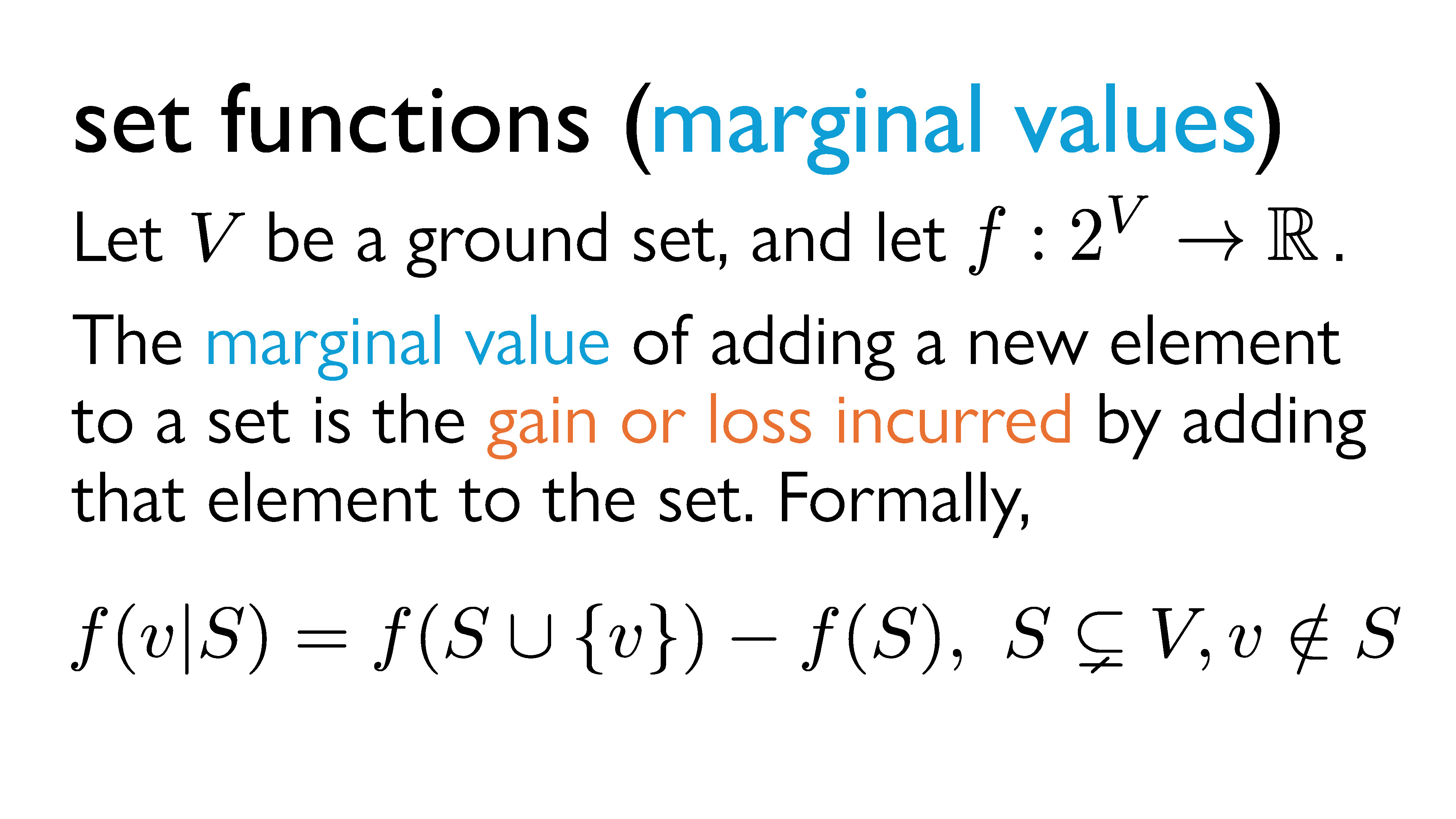
Another term that will be extremely useful for us is the concept of marginal values. The marginal value of adding a new element to a set is the gain or loss incurred by adding that element to the set. There are many equivalent notations for this, but we will denote this \(f(v|S)\) (read “the marginal value of \(v\) to \(S\)”).
Formally, for a set \(S\) and an element \(v\), \(f(v|S) = f(S \cup \\{v\\}) - f(S)\), where \(S \subsetneq V\) and \(v \notin S\).
Marginal utility

Before I formally explain this modularity business, I want to take a brief interlude to explain a concept from economics that really helped these ideas make more concrete sense to me. This concept is called marginal utility. It refers to the extra value you get from having one additional unit of something. If we use pizza slices as an example, if you are very hungry, the first pizza slice you eat will have a very high value, because it will satiate your hunger. But subsequent pizza slices will have less value, because you won’t be as hungry anymore. If you eat too many slices, you might even feel sick, so that last slice would actually have negative value. So each slice of pizza you eat actually has diminishing returns, and most consumer goods follow something called the law of diminishing returns. However, diminishing marginal utility doesn’t apply in every scenario. For example, if we take bricks as an example, a single brick isn’t particularly useful on its own, and neither is a set of two or three bricks. However, a set of a million bricks is actually useful, because you can build something. So in the case of bricks, you actually get increasing returns with each new brick. (Well, not strictly – but this example is good enough for our purposes.)
Lastly, you can also have constant returns. For example, every single dollar has the same value. This means that every dollar you add to your bank account increases your purchasing power by the same amount.
We’ll formalize this notion a bit in a second, but abstractly, a submodular function is a set function characterized by diminishing returns. (You may be completely unsurprised to hear that economics really seem to like this concept.) A supermodular function is characterized by increasing returns, and a modular function is characterized by constant returns.
Submodular, Supermodular, and Modular Functions: Formal Definitions
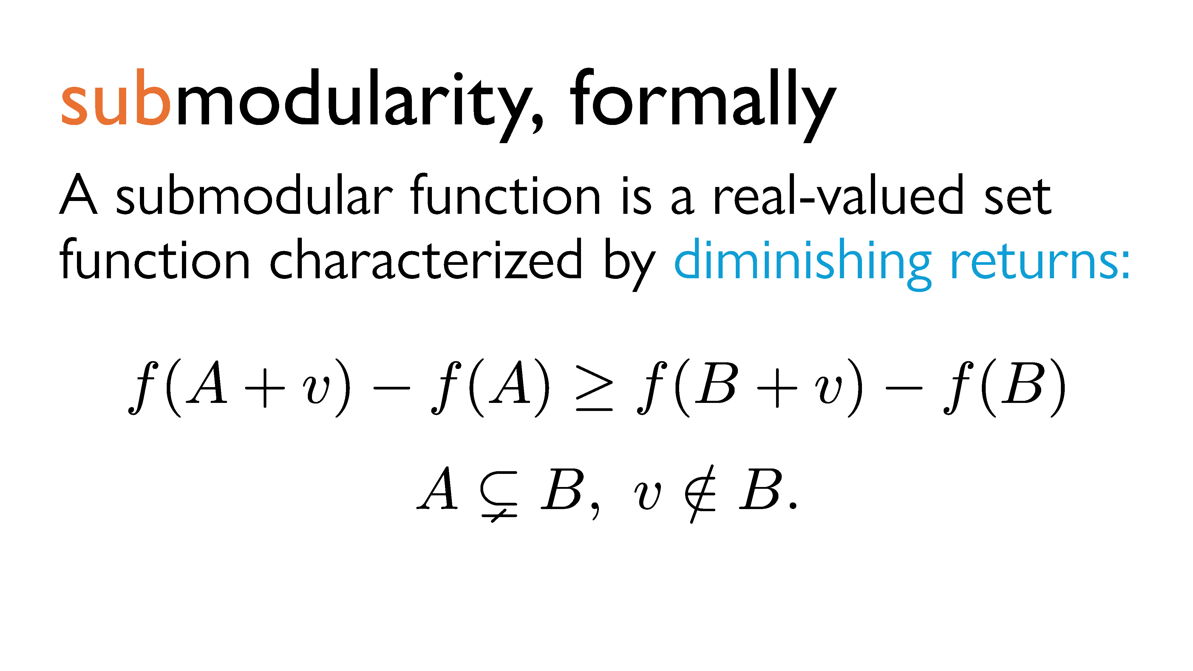
A submodular function is a real-valued set function characterized by diminishing returns. In other words, a very informal way to look at it is that the marginal value of \(v\) to \(S\) decreases as the number of elements in \(S\) increases. Or, if \(A\) is a (strict) subset of \(B\), then adding \(v\) to \(A\) will induce a greater (or equal) change in value than adding \(v\) to \(B\).
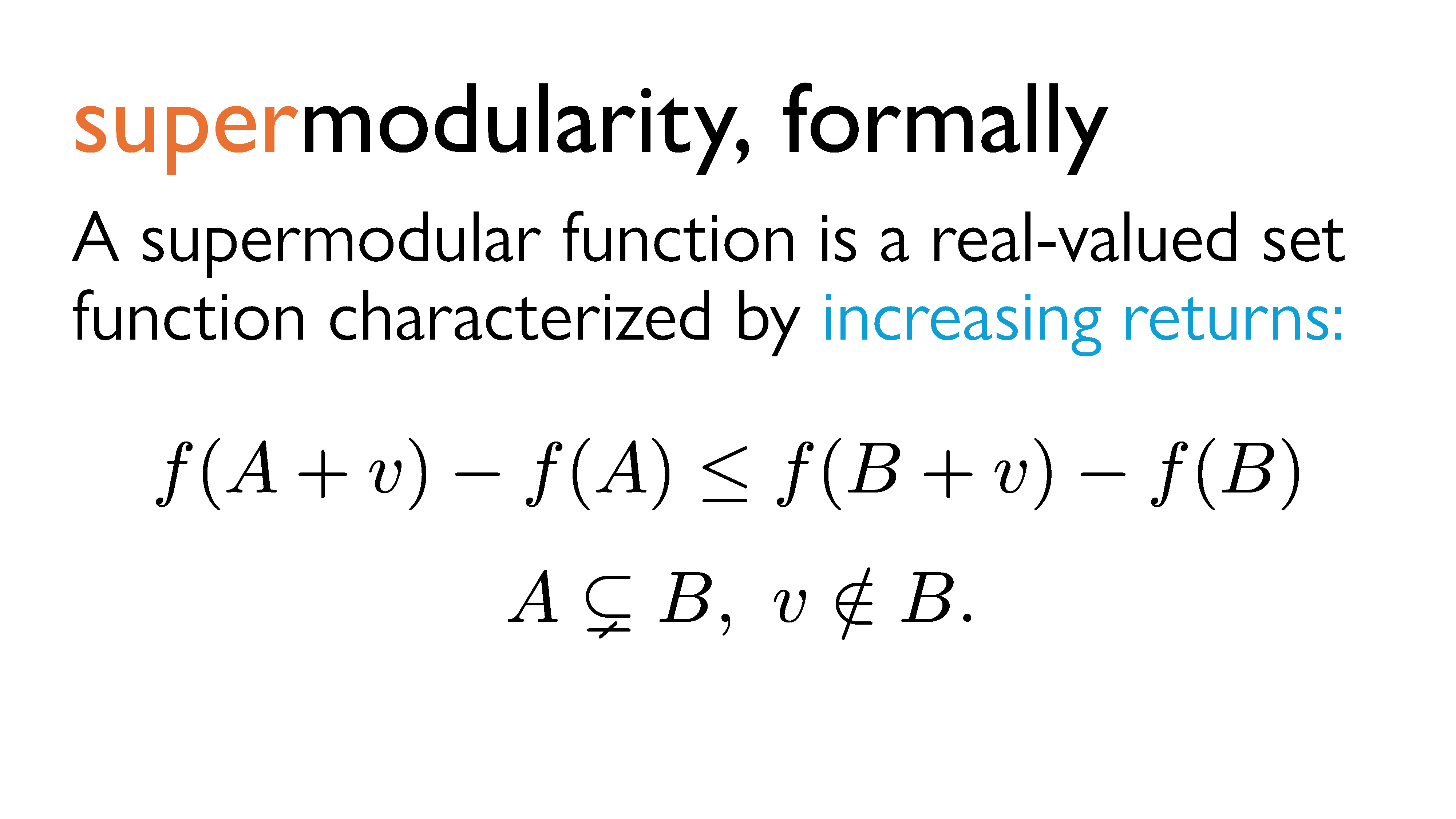
A supermodular function is a real-valued set function characterized by increasing returns. In other words, a very informal way to look at it is that the marginal value of \(v\) to \(S\) increases as the number of elements in \(S\) increases. Or, if \(A\) is a (strict) subset of \(B\), then adding \(v\) to \(A\) will induce a lesser (or equal) change in value than adding \(v\) to \(B\).
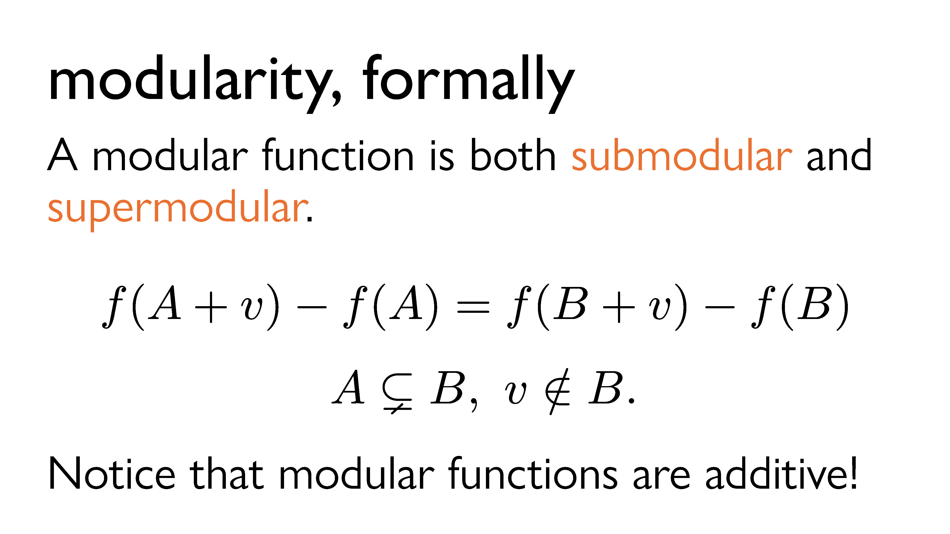
If a function is both submodular and supermodular, then we call it a modular function. Modular functions are characterized by constant returns. It’s worth noting that this implies that modular set functions are always additive.
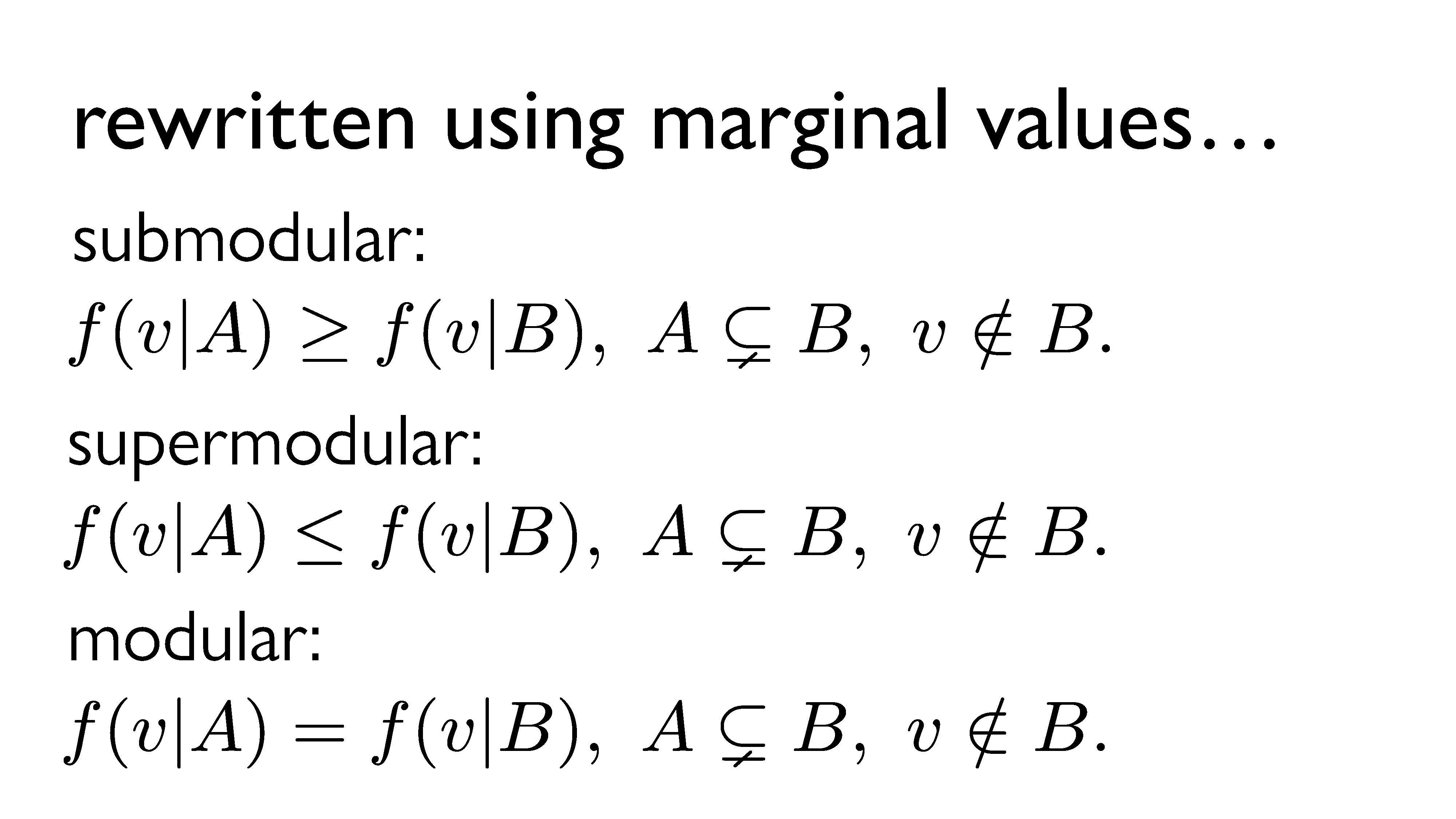
In summary, for \(A \subsetneq B\), a set function \(f\) is submodular if \(f(v|A) \geq f(v|B)\), supermodular if \(f(v|A) \leq f(v|B)\), and modular if \(f(v|A) = f(v|B)\).
Generalization: The Densest Supermodular Set Problem (DSSP)
In part 3 of this talk, we discussed the densest subgraph problem (DSP) and some approximation algorithms for solving it. I then mentioned that by generalizing the problem even further, we might be able to solve some other problems. This generalization is known as the densest supermodular set problem (DSSP). First, we’ll take a look at what the DSSP actually is; then, we’ll discuss how it applies to both the DSP and potential related problems.
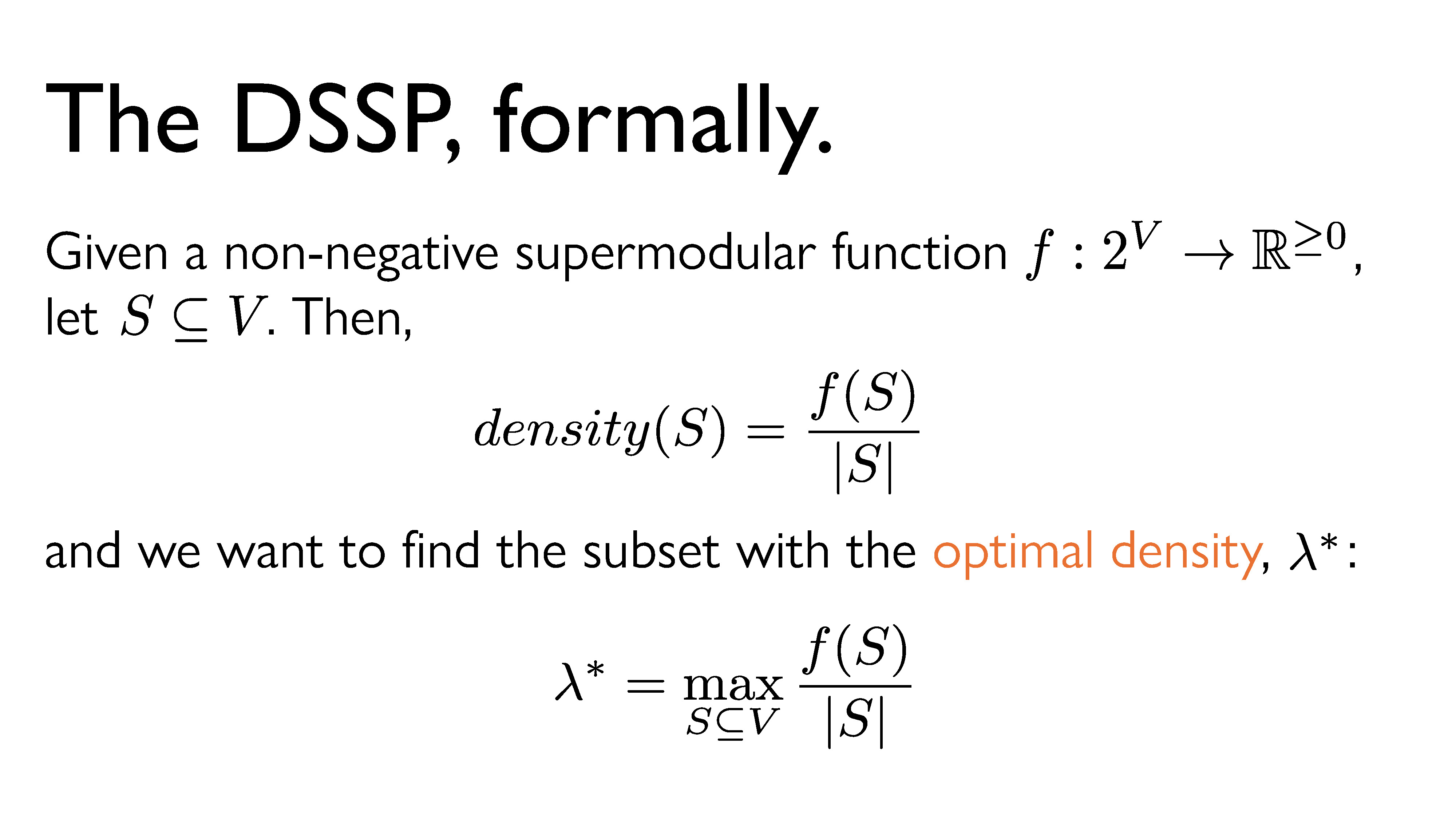
Here’s a somewhat formal statement of the DSSP. First, we define some ground set \(V\), and a set function \(f: 2^V \rightarrow \mathbb{R}^{\geq 0}\). For any subset \(S\) of \(V\), we define its density to be its value under \(f\) divided by its size. That is, \(density(S) = \frac{f(S)}{|S|}\). Now, we want to find the subset that maximizes the density. We’re going to call that density the the optimal density and denote it \(\lambda^*\). Now, this might all sound very abstract. What’s up with all these sets? What is this supermodular function, and how can we use it to optimize anything? But remember, a supermodular function just assigns values to subsets in such a way that they exhibit the increasing returns property. As an example, it’s worth noting that our induced-edge counting function from earlier, \(|E(S)|\), is actually supermodular. Let’s let \(f = |E(S)|\), where \(S\) is a set of vertices in a graph.
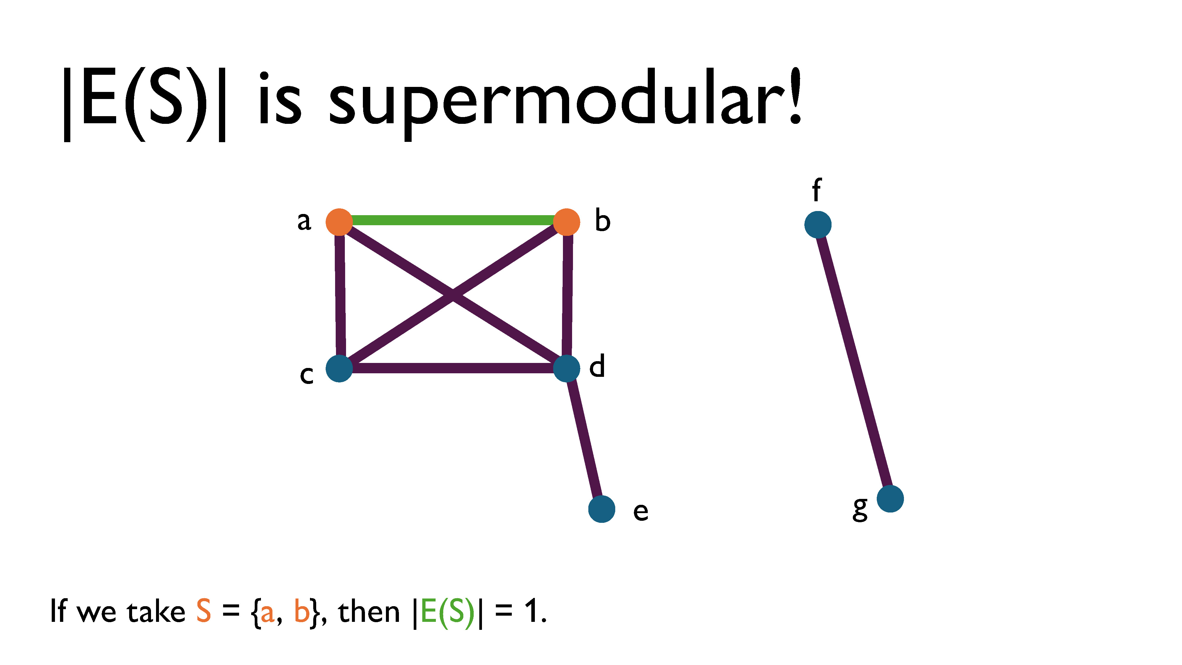
If we look at the example graph above, we see that if we take \(S = \\{a, b\\}\), then \(|E(S)| = 1\).
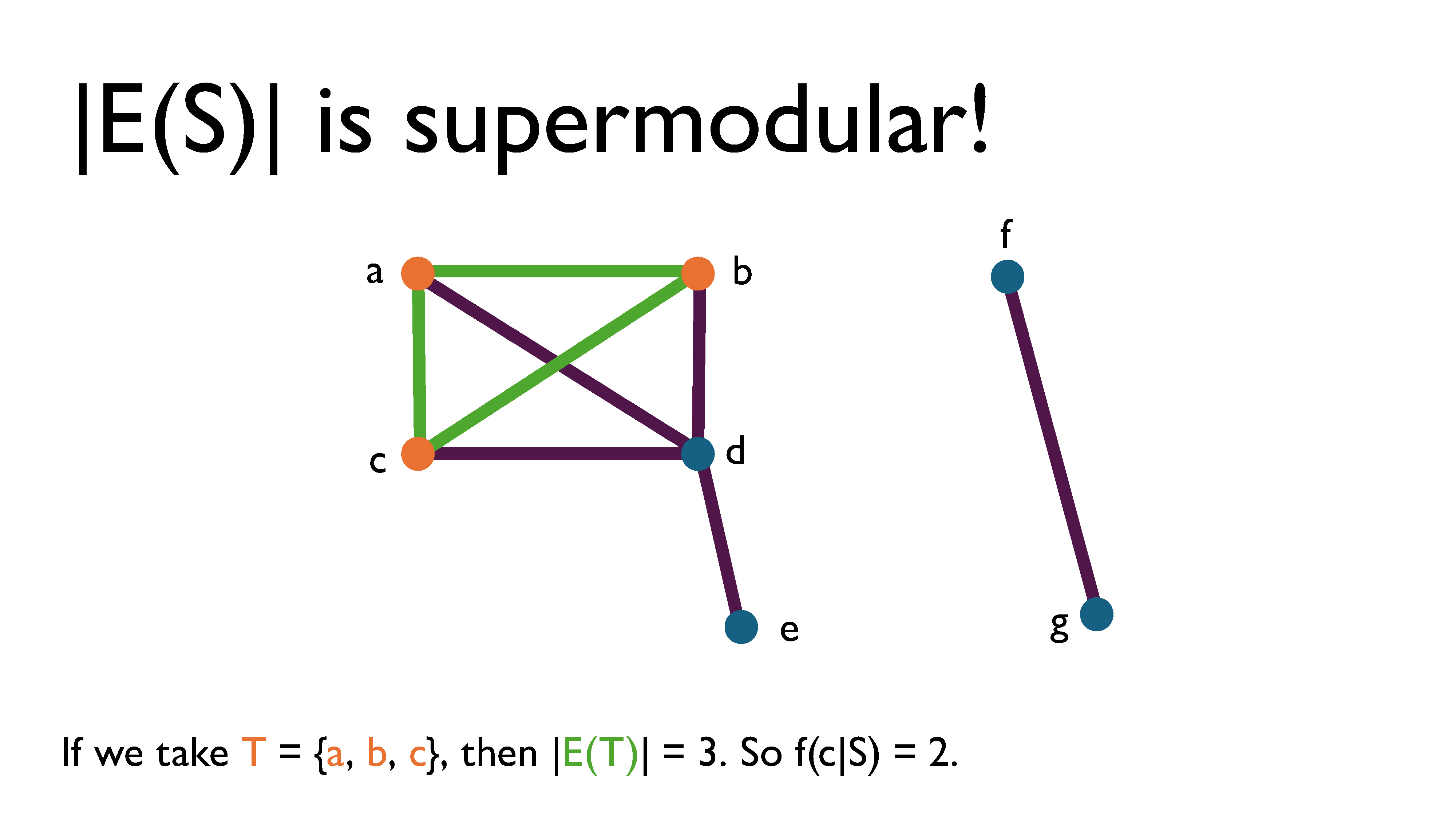
If we take \(T = \\{a, b, c\\}\), then \(|E(T)| = 3\). So \(f(c|S) = 2\).
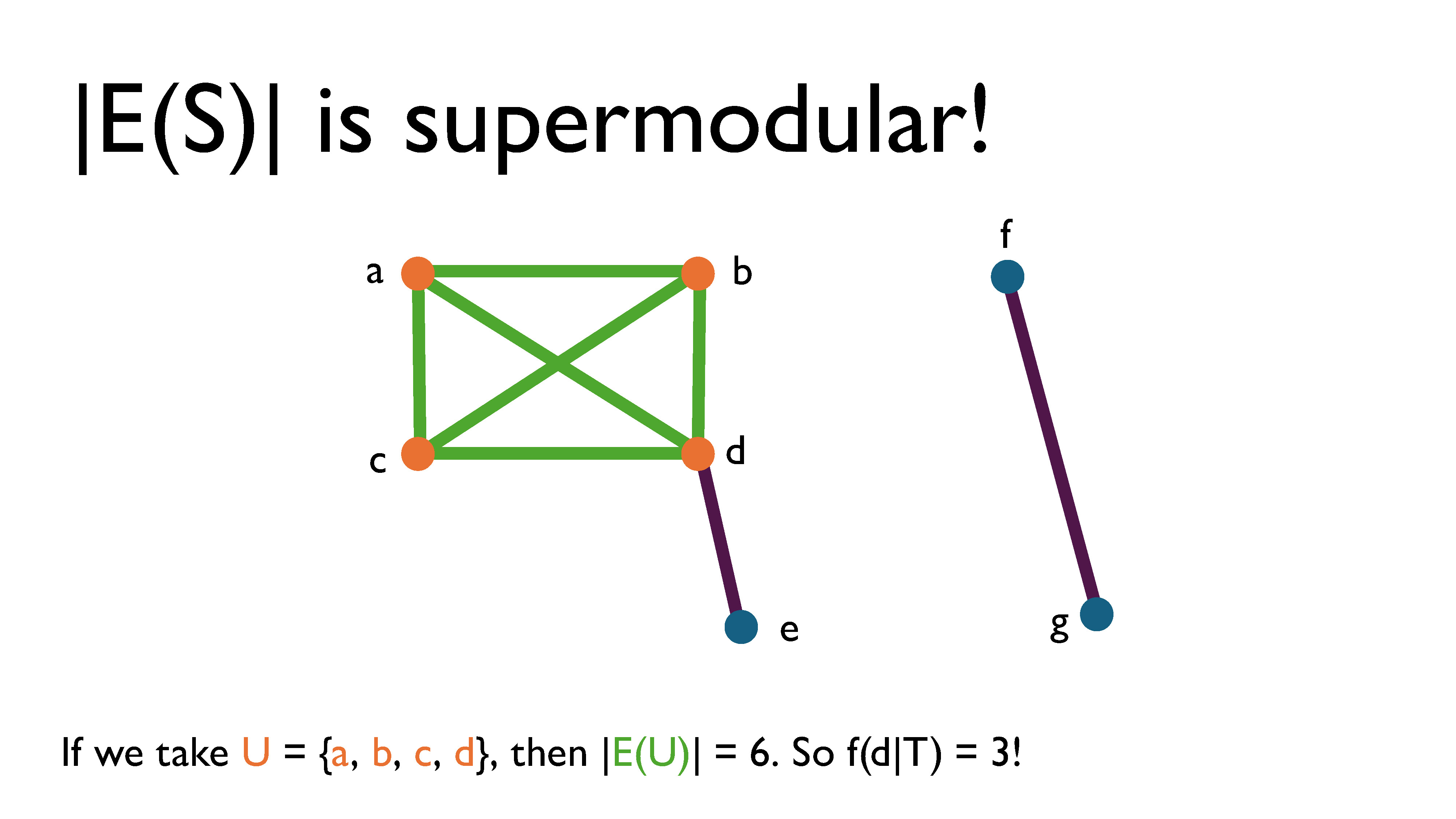
If we take \(U = \\{a, b, c, d\\}\), then \(|E(U)| = 6\). So \(f(d|T) = 3\). This clearly shows that this function has increasing returns, which intuitively makes sense; the more vertices are in the subgraph, the more edges can be included in the induced graph by adding another vertex.
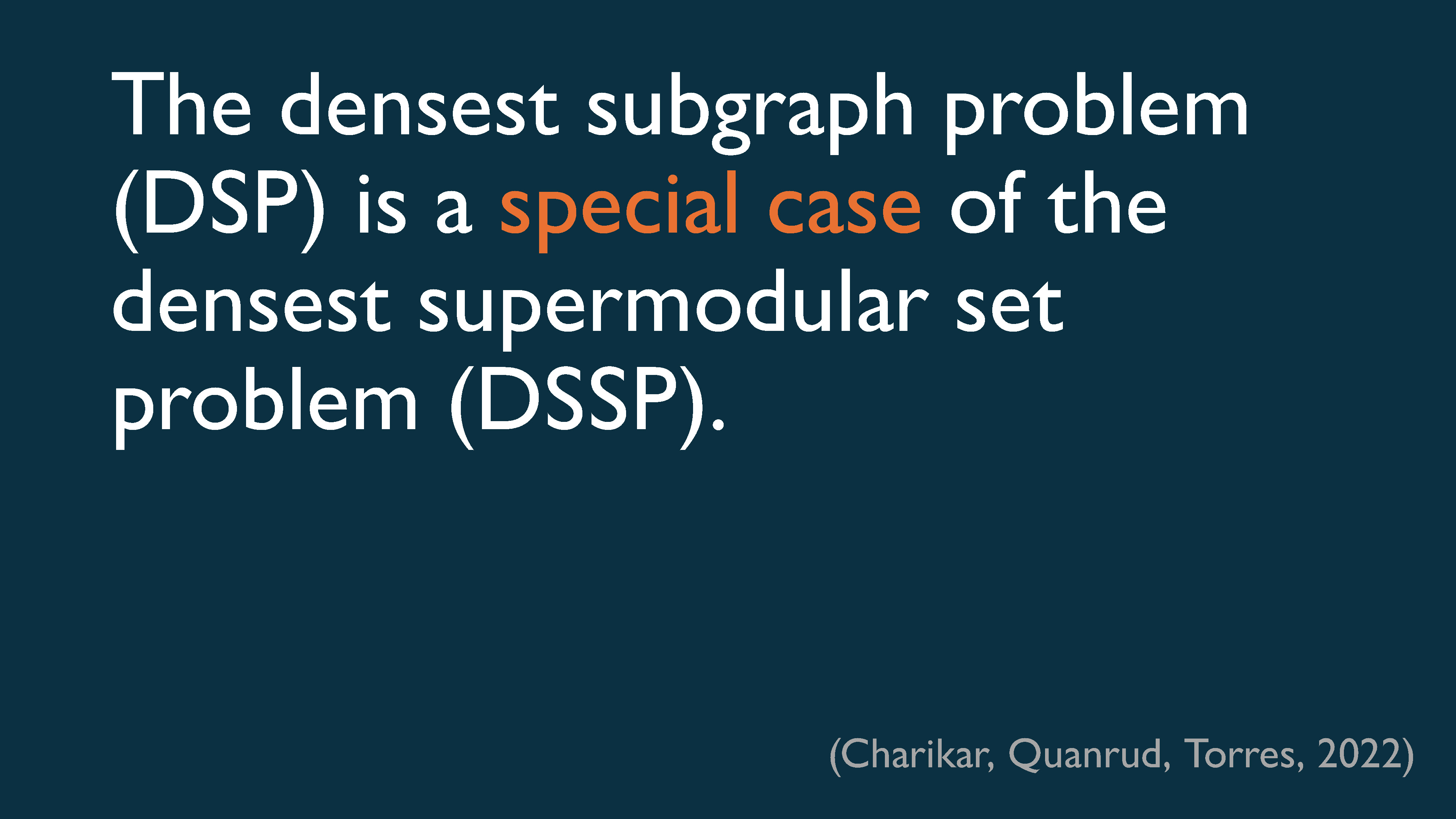
Subbing in \(|E(S)|\) for \(f(S)\) then, it’s clear that the DSP is a special case of the DSSP.
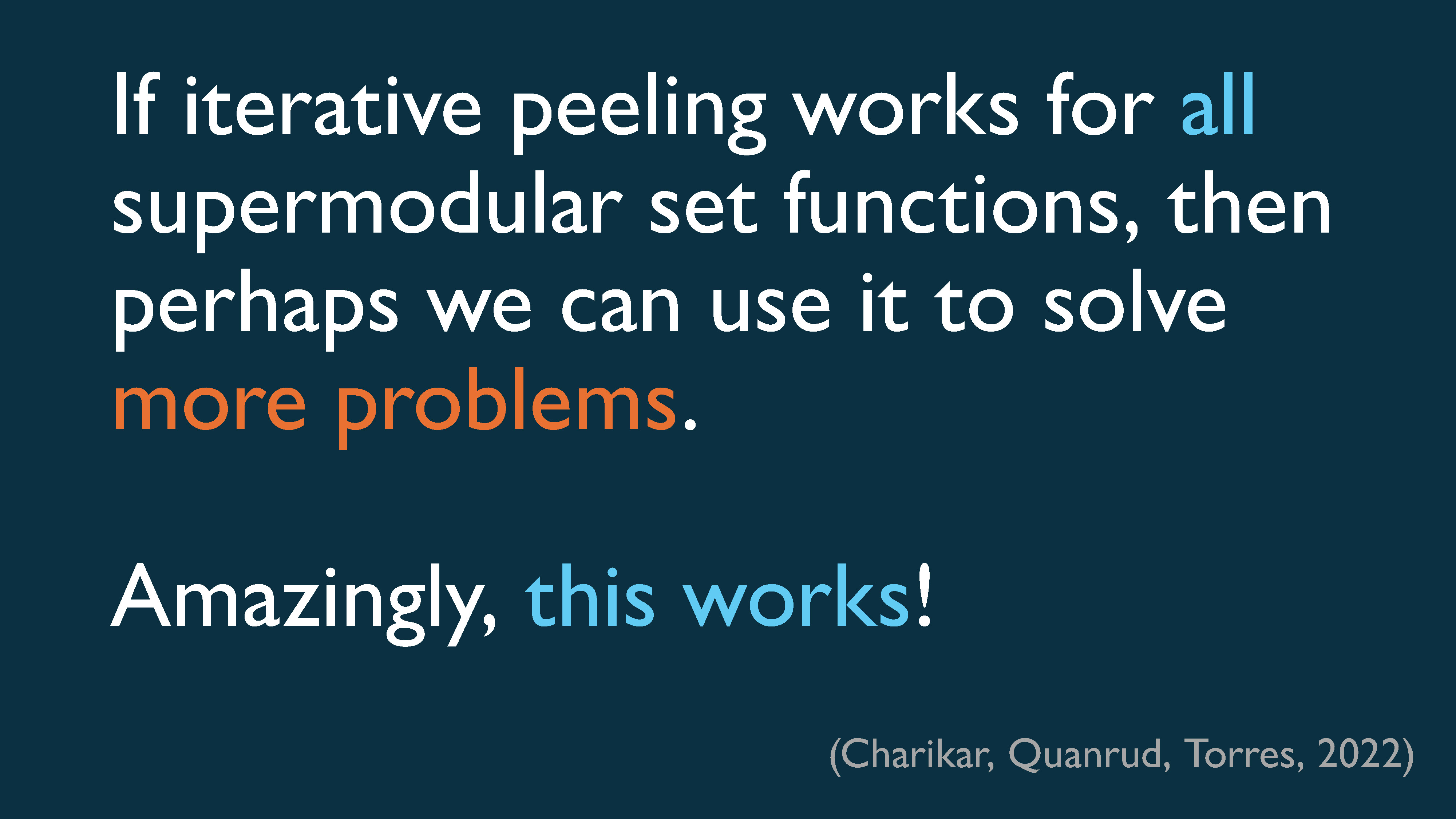
Now, if we were somehow able to generalize iterative peeling to work for all supermodular set functions, then perhaps we could use it to solve a lot more problems than just the DSP. Amazingly, this was shown to work by Charikar, Quanrud, and Torres in their 2022 paper (link here). They called the iterative peeling algorithm for supermodular set functions SuperGreedy++3.
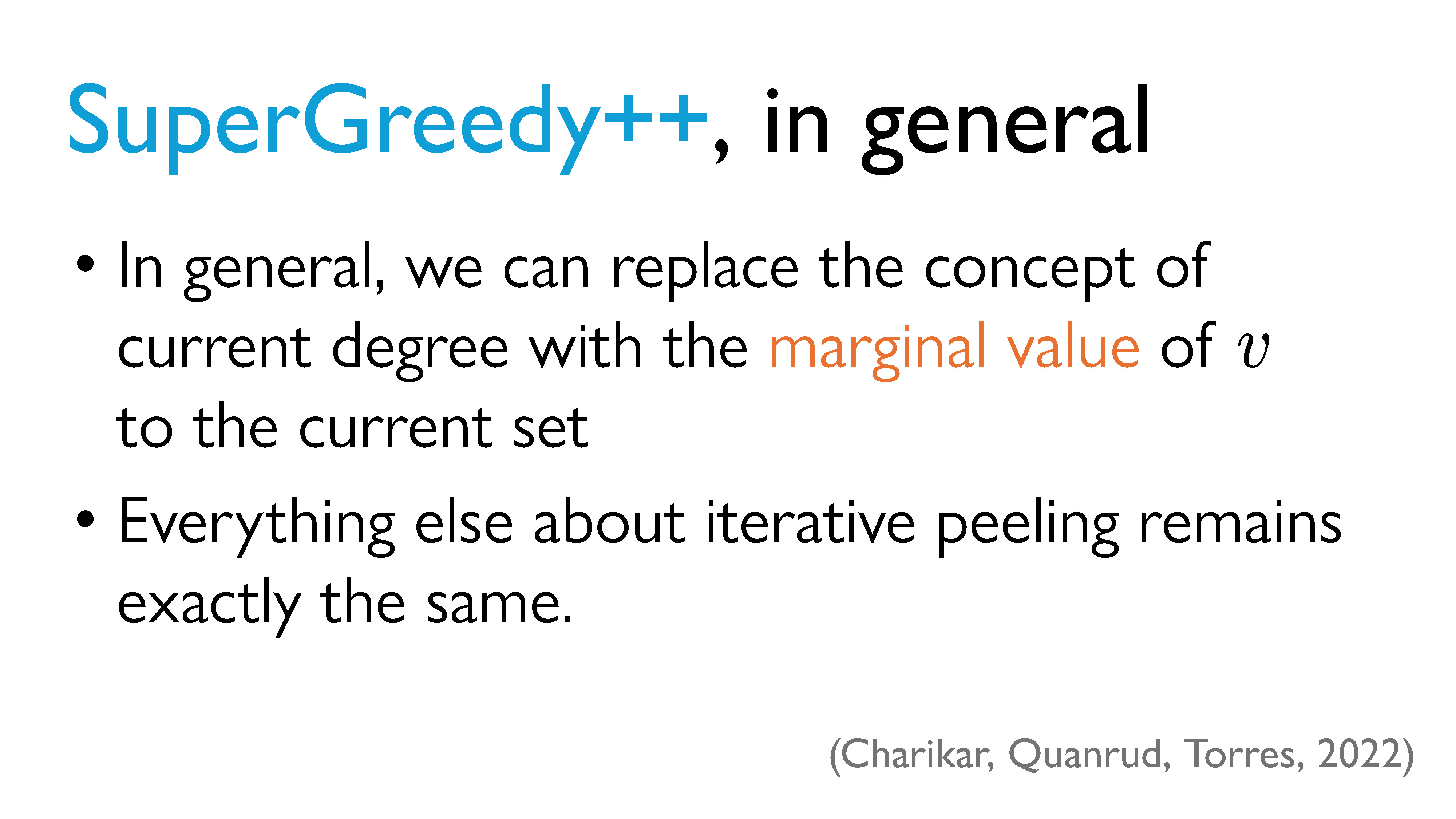
In general, for supermodular set functions, we just peel based on the marginal values of elements to the current set instead of peeling based on the degree of a vertex. (In fact, if our function is \(|E(S)|\), then the current degree of some vertex \(v\) in \(S\) is actually its marginal value to \(S\)). Everything else about peeling stays the same.
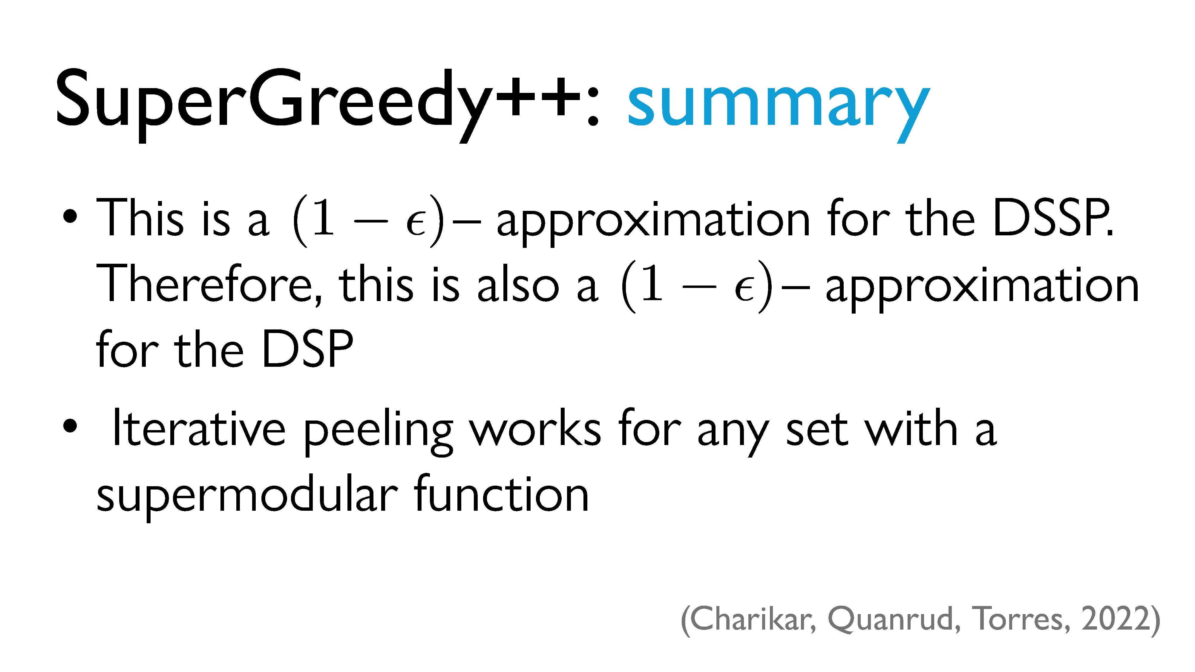
Iterative peeling works for any set with a supermodular function. Chekuri, Quanrud, and Torres also showed that SuperGreedy++ is a \((1-\epsilon)\)–approximation to the DSSP. What this means, very roughly, is that you can get as close as you want to the optimal answer so long as you’re willing to run enough iterations (and the number of iterations required depends on how small you decide your error tolerance is). This also tells us that it’s a \((1-\epsilon)\)–approximation to the DSP.
Key Takeaways
So what did we learn from all of this? There were many detours, but overall, I hope you were able to get a sense of how we can use theoretical approaches to come up with solutions to problems.
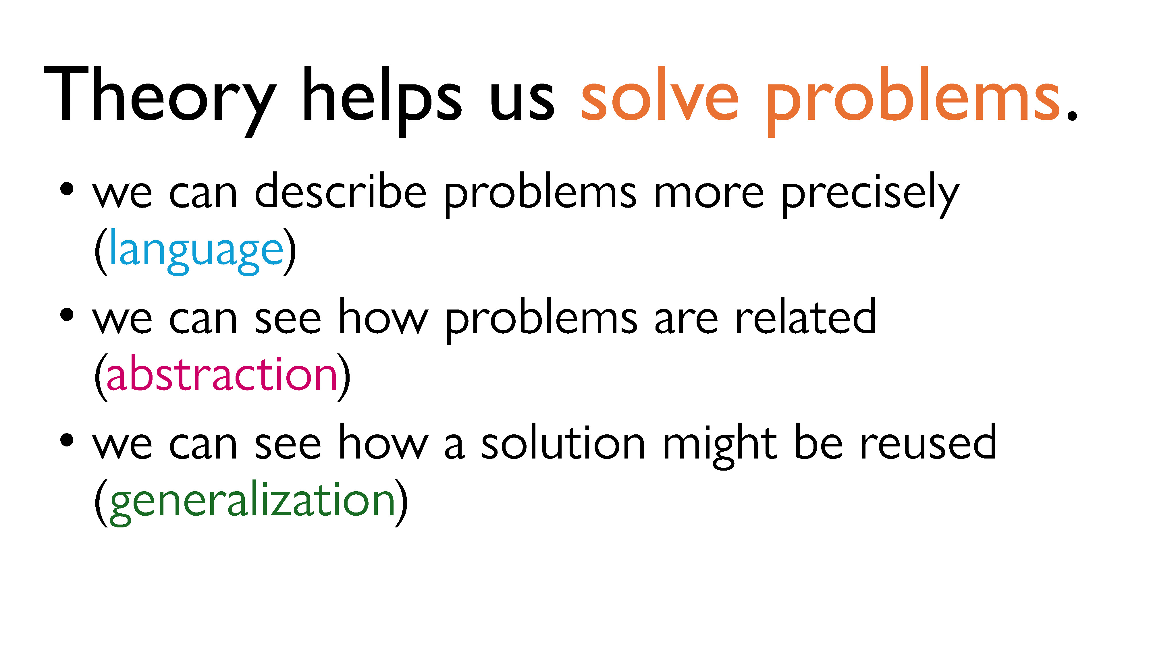
There are three main things I’d like you to take away from this series:
- Theory is useful because it helps us develop language to describe problems more precisely.
- Theory helps us understand how different problems are related, through the use of abstraction.
- Theory helps us find ways to reuse existing solutions or approaches, through the use of generalization.
Lastly, I hope you gained a little bit more of an appreciation for math4. I know I may have lost some of you part of the way through the formalism and minutiae, and that’s okay. But I hope you understand that these abstractions aren’t just some pointless thing mathematicians make us learn to make their field seem more legitimate. They can actually be useful in concrete ways, sometimes5.
Part 5: References, Resources, and Further Reading
Here is a long list of sources I consulted at various points while doing research for this project. As it might have become clear through reading the previous installments of this series, this was more a talk about the densest subgraph problem than it was about theory being useful in computer science. There are a few reasons for that, which I might explain in more detail at some point in the future6. This means that I presented a lot of information that I borrowed from other people! Here’s an annotated bibliography of sorts, in case you were interested in going deeper, for whatever reason.
Key Sources I Consulted
Chandra Chekuri’s invited talk at the Tutte Seminar, University of Waterloo C&O department
Link: https://www.youtube.com/watch?v=DO8iNCwmp0c
In this talk, Chekuri talks about the paper he coauthored that had to do with iterative peeling. I found it very helpful to watch this video (very slowly) while trying to decipher the paper7.
Jeff A. Bilmes: Deep mathematical properties of submodularity with applications to machine learning
Link: https://www.youtube.com/watch?v=ZycBUGLD22E
This is a two-hour long tutorial about submodularity that Jeff Bilmes presented at Microsoft Research in 2016. I have no idea how I found this (maybe I just started searching “submodularity” on YouTube or something), but it was a total godsend. I owe so much to this video: it filled in gaps I didn’t know I had and provided context I wouldn’t have known how to look for. The amount of information condensed into this video is truly impressive, and I spent many, many more than two hours watching and trying to digest it.
Bilmes also teaches a course on this, and I referenced his course notes a few times. Here’s the link: https://people.ece.uw.edu/bilmes/classes/ee563/ee563_fall_2020/
Background and other Links
- Vital Sine’s YouTube series on Hypergraph Theory: https://youtube.com/playlist?list=PLZ2xtht8y2-IRjvXJJpka2GIJ3wn7u4g2
- Jonatan Lindén’s technical report on Hypergraphs and Matroids: https://perso.ens-lyon.fr/eric.thierry/Graphes2007/jonatan-linden.pdf
- The Wikipedia article on set functions: https://en.wikipedia.org/wiki/Set_function
- The Wolfram alpha entry on set functions: https://mathworld.wolfram.com/SetFunction.html
- Notes on submodular optimization from CS 880: Approximation and Online Algorithms, University of Wisconsin: https://pages.cs.wisc.edu/~shuchi/courses/880-F19/
- Notes on Minimum Cuts and Modular Functions: https://www.robots.ox.ac.uk/~pankaj/notes/notes_cunningham.pdf
- Cornell University, CS 6280: Algorithms - Bobby Kleinberg’s notes on Submodular functions: https://www.cs.cornell.edu/courses/cs6820/2019fa/handouts/submod.pdf
- Chekuri’s Notes from his Approximation Algorithms course (CS 583, Spring 2018, Introduction Lecture): https://courses.grainger.illinois.edu/cs583/sp2018/Notes/intro.pdf
- Cornell University Computational Optimization Open Textbook, Heuristic Algorithms page: https://optimization.cbe.cornell.edu/index.php?title=Heuristic_algorithms
- The Wikipedia article on heuristics: https://en.wikipedia.org/wiki/Heuristic_(computer_science)
- Local Search Algorithms in AI: A Comprehensive Guide: https://www.simplilearn.com/local-search-algorithms-in-ai-article
- Wikipedia article on Relaxations: https://en.wikipedia.org/wiki/Relaxation_(approximation)
- Charalampos E. Tsourakakis and Tianyi Chen, Dense subgraph discovery (DSD) theory and applications: https://tsourakakis.com/dense-subgraph-discovery-theory-and-applications-tutorial-sdm-2021/
- Jan Vondrák, Continuous extensions of submodular functions: https://theory.stanford.edu/~jvondrak/CS369P/lec17.pdf
Academic Papers
A Survey on the Densest Subgraph Problem and its Variants (2024)
Authors: Tommaso Lanciano, Atsushi Miyauchi, Adriano Fazzone, and Francesco Bonchi
DOI: https://doi.org/10.1145/3653298
ArXiv Link: https://arxiv.org/abs/2303.14467
This is an academic paper that covers pretty much everything that’s been published about the densest subgraph problem (except for some very recent stuff).
Greedy approximation algorithms for finding dense components in a graph (2000)
Author: Moses Charikar
DOI: https://doi.org/10.1007/3-540-44436-X_10
here’s a link to a PDF
An academic paper about a greedy “peeling” algorithm for solving the DSP. This paper is very famous.
Flowless: Extracting Densest Subgraphs Without Flow Computations (2020)
Authors: Digvijay Boob, Yu Gao, Richard Peng, Saurabh Sawlani, Charalampos E. Tsourakakis, Di Wang, Junxing Wang
DOI: https://doi.org/10.1145/3366423.3380140
ArXiv Link: https://arxiv.org/abs/1910.07087
This is the original paper on “iterative peeling” for the DSP (Greedy++). These authors also ran a bunch of tests with real data to show how the algorithm performed.
Densest Subgraph: Supermodularity, Iterative Peeling, and Flow (2022)
Authors: Chandra Chekuri, Kent Quanrud, and Manuel R. Torres
DOI: https://doi.org/10.1137/1.9781611977073.64
PDF on Author’s Website: https://chekuri.cs.illinois.edu/papers/densest-subgraph-soda22.pdf
This is the paper that first uses supermodularity to study the DSP and iterative peeling through defining the “densest supermodular set problem”. This is where the algorithm SuperGreedy++ came from. The authors also analyze SuperGreedy++ and prove that it converges to a (1–epsilon)-approximation for the DSP. This paper also contains a bunch of other stuff that I didn’t look into too deeply.
Submodular functions and convexity (1983)
Author: László Lovász
DOI: https://doi.org/10.1007/978-3-642-68874-4_10
I read this paper because I was trying to retrace the origins of the “Lovász extension” and understand what it means. This is the original paper that talks about the links between submodularity, convexity, and concavity.
Submodular function minimization (2013)
Author: S. Thomas McCormick
Link: https://www.lamsade.dauphine.fr/~poc/jpoc8/McCormick-fcts-ss-modulaires.pdf
DOI (earlier version): https://doi.org/10.1016/S0927-0507(05)12007-6
This book chapter is a very complete introduction to submodular function minimization and I stole all sorts of stuff from it. Importantly, it contains a proof that the two definitions of submodularity are equivalent, which I very much appreciated seeing.
On finding dense subgraphs (2009)
Authors: Samir Khuller and Barna Saha
DOI: https://doi.org/10.1007/978-3-642-02927-1_50
PDF on Author’s Website: https://www.cs.umd.edu/~samir/grant/ICALP09.pdf
I think I looked at a proof technique or two in this paper? Honestly, I don’t remember anymore. What I can say is that it provides an alternative proof of a claim in Charikar’s 2000 paper (mentioned above)
Authoritative sources in a hyperlinked environment (1999)
Author: Jon M. Kleinberg
DOI: https://doi.org/10.1145/324133.324140
PDF: https://dl.acm.org/doi/pdf/10.1145/324133.324140
One of the sources I cited in my short survey of “real-world problems” in Part 2.
Studying complex discursive systems (2002)
Authors: Steven R. Corman, Timothy Kuhn, Robert D. McPhee, and Kevin J. Dooley
DOI: https://doi.org/10.1111/j.1468-2958.2002.tb00802.x
Another source I cited in my short survey of “real-world problems” in Part 2. This one is the linguistics paper that refers to a technique called “centering resonance analysis”.
Dense subgraph extraction with application to community detection (2012)
Authors: Jie Chen and Yousef Saad
DOI: https://doi.org/10.1109/TKDE.2010.271
Yet another source I cited in my short survey of “real-world problems” in Part 2.
Footnotes
This algorithm is usually attributed to the researcher Moses Charikar and is commonly known in the research community as “Charikar’s greedy algorithm” or “Charikar’s peeling algorithm”. That being said, the Japanese scientists Yuichi Asahiro, Kazuo Iwama, Hisao Tamaki, and Takeshi Tokuyama used pretty much the same algorithm in a slightly different context back in 1996. While it is known that they are the ones who came up with this idea, I just find it interesting to examine who it is who actually gets named credit for things, because it’s not always the actual originator of the idea who gets credit.↩︎
This notation comes from set theory, and means the set of all functions from \(S\) to some two-element set, usually taken to be the set \(\\{0,1\\}\). This set is isomorphic to the powerset of \(S\), so the two are often used interchangeably. (Honestly, I’m not 100% sure why the authors of the papers I’ve been reading decided to use this notation instead, but after using it myself, I have to say I also prefer it and will likely adopt it too. It’s just… cleaner, I guess.)↩︎
Incidentally, iterative peeling for graphs is called Greedy++. Computer scientists are clearly very creative with their naming skills.↩︎
Although, if you ask the average mathematician, this is the kind of math that is mostly interesting to computer scientists. So really, I hoped you gained more of an appreciation for theoretical computer science.↩︎
It is true that there is a lot of highly specialized math that doesn’t seem to have any concrete applications. However, as far as I can tell, a lot of that math isn’t actually being taught to undergraduates. Most math taught in undergrad, even the abstract “pure” math taught to math majors, has real applications. The actual problem is that there are some math professors who aren’t actually interested in talking about applications. Every once in a while, someone who is 100% theoretically inclined teaches what is supposed to be an applied course, which can be frustrating if you care about applications.↩︎
The short version is that I’d been wanting to give a talk about the importance of theory in CS for a long time, and I’d also been wanting to talk about the evolution of algorithms for solving the DSP. However, I was also taking a course where I had to give a technical presentation on algorithms for the DSP the day after I was giving this talk, so I decided to make the first half of it mostly about the important of theory and make the second half be somewhat practice for my presentation the next day. Now, this is a terrible way to give a coherent talk (and I’m sure it felt like I was giving two talks), but I didn’t think I’d get any other chances to give a talk that year, so I did what I felt like I had to do.↩︎
I kid you not, I found a PDF of his slides, slowed the video down to 0.75 speed, and wrote down what he said almost word for word, which helped fill in some gaps. The key thing to note is that papers tend to assume the reader has the exact same background as the author – talks usually don’t, so they include quite a bit more context. Not enough that I could actually understand what was happening without prior background, but enough that I could begin to stumble through things and figure out what sort of things to look up.↩︎